Repository of Reproducible Computations

Free Statistics

of Irreproducible Research!

Author's title

Author

*Unverified author*

R Software Module

rwasp_autocorrelation.wasp

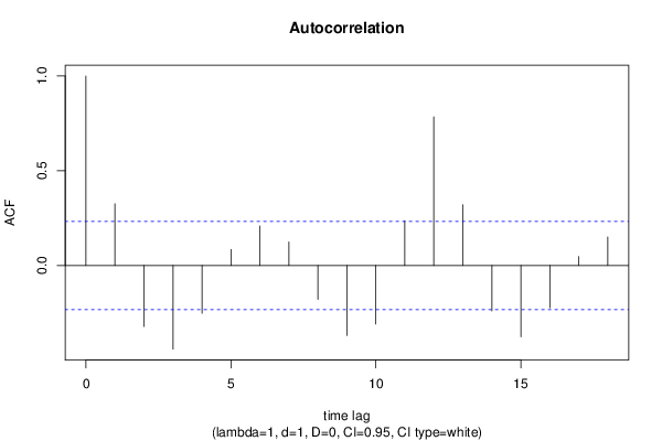
Title produced by software

(Partial) Autocorrelation Function

Date of computation

Fri, 17 Oct 2014 09:36:37 +0100

Cite this page as follows

Statistical Computations at FreeStatistics.org, Office for Research Development and Education, URL https://freestatistics.org/blog/index.php?v=date/2014/Oct/17/t1413535010lfiny6uj5bln9iz.htm/, Retrieved Fri, 10 May 2024 07:30:42 +0000

Statistical Computations at FreeStatistics.org, Office for Research Development and Education, URL https://freestatistics.org/blog/index.php?pk=243186, Retrieved Fri, 10 May 2024 07:30:42 +0000

QR Codes:

Paste this QR Code to cite your computation.

Original text written by user:

IsPrivate?

No (this computation is public)

User-defined keywords

Eline Van Loon

Estimated Impact

130

Family? (F = Feedback message, R = changed R code, M = changed R Module, P = changed Parameters, D = changed Data)

-       [(Partial) Autocorrelation Function] [] [2014-10-17 08:36:37] [9adebd9d8505f0d6c7bd6ecbde218cd8] [Current]
- R P     [(Partial) Autocorrelation Function] [] [2014-11-13 10:27:56] [021f24b0772399b3b291bd2200abf137] 
- RMPD    [Bootstrap Plot - Central Tendency] [] [2014-11-13 14:49:32] [021f24b0772399b3b291bd2200abf137] 
- RMPD    [Bootstrap Plot - Central Tendency] [] [2014-11-13 14:52:59] [021f24b0772399b3b291bd2200abf137] 
- RMPD    [Bootstrap Plot - Central Tendency] [] [2014-11-13 14:56:25] [021f24b0772399b3b291bd2200abf137] 
- RMP     [Blocked Bootstrap Plot - Central Tendency] [] [2014-11-13 15:53:40] [021f24b0772399b3b291bd2200abf137] 
- RMP     [Blocked Bootstrap Plot - Central Tendency] [] [2014-11-13 15:57:07] [021f24b0772399b3b291bd2200abf137] 
- RMP     [Blocked Bootstrap Plot - Central Tendency] [] [2014-11-13 16:00:25] [021f24b0772399b3b291bd2200abf137] 

Feedback Forum

Post a new message

Dataseries X:

Download CSV

Histogram

Boxplots

Summary of computational transaction
Raw Input	view raw input (R code)
Raw Output	view raw output of R engine
Computing time	1 seconds
R Server	'Gwilym Jenkins' @ jenkins.wessa.net

\begin{tabular}{lllllllll}
\hline
Summary of computational transaction \tabularnewline
Raw Input & view raw input (R code)  \tabularnewline
Raw Output & view raw output of R engine  \tabularnewline
Computing time & 1 seconds \tabularnewline
R Server & 'Gwilym Jenkins' @ jenkins.wessa.net \tabularnewline
\hline
\end{tabular}
%Source: https://freestatistics.org/blog/index.php?pk=243186&T=0

[TABLE]
[ROW][C]Summary of computational transaction[/C][/ROW]
[ROW][C]Raw Input[/C][C]view raw input (R code) [/C][/ROW]
[ROW][C]Raw Output[/C][C]view raw output of R engine [/C][/ROW]
[ROW][C]Computing time[/C][C]1 seconds[/C][/ROW]
[ROW][C]R Server[/C][C]'Gwilym Jenkins' @ jenkins.wessa.net[/C][/ROW]
[/TABLE]
Source: https://freestatistics.org/blog/index.php?pk=243186&T=0

Globally Unique Identifier (entire table): ba.freestatistics.org/blog/index.php?pk=243186&T=0

As an alternative you can also use a QR Code:

The GUIDs for individual cells are displayed in the table below:

Summary of computational transaction
Raw Input	view raw input (R code)
Raw Output	view raw output of R engine
Computing time	1 seconds
R Server	'Gwilym Jenkins' @ jenkins.wessa.net

Autocorrelation Function
Time lag k	ACF(k)	T-STAT	P-value
1	0.325583	2.7434	0.003846
2	-0.322028	-2.7135	0.004175
3	-0.441229	-3.7179	0.000199
4	-0.252003	-2.1234	0.018603
5	0.084468	0.7117	0.23948
6	0.208426	1.7562	0.041681
7	0.124265	1.0471	0.149309
8	-0.179031	-1.5085	0.067926
9	-0.369383	-3.1125	0.001337
10	-0.308861	-2.6025	0.005629
11	0.235981	1.9884	0.025311
12	0.784013	6.6062	0
13	0.320815	2.7032	0.004293
14	-0.23976	-2.0203	0.023566
15	-0.376698	-3.1741	0.001111
16	-0.223083	-1.8797	0.032124
17	0.046723	0.3937	0.347492
18	0.150344	1.2668	0.10468

\begin{tabular}{lllllllll}
\hline
Autocorrelation Function \tabularnewline
Time lag k & ACF(k) & T-STAT & P-value \tabularnewline
1 & 0.325583 & 2.7434 & 0.003846 \tabularnewline
2 & -0.322028 & -2.7135 & 0.004175 \tabularnewline
3 & -0.441229 & -3.7179 & 0.000199 \tabularnewline
4 & -0.252003 & -2.1234 & 0.018603 \tabularnewline
5 & 0.084468 & 0.7117 & 0.23948 \tabularnewline
6 & 0.208426 & 1.7562 & 0.041681 \tabularnewline
7 & 0.124265 & 1.0471 & 0.149309 \tabularnewline
8 & -0.179031 & -1.5085 & 0.067926 \tabularnewline
9 & -0.369383 & -3.1125 & 0.001337 \tabularnewline
10 & -0.308861 & -2.6025 & 0.005629 \tabularnewline
11 & 0.235981 & 1.9884 & 0.025311 \tabularnewline
12 & 0.784013 & 6.6062 & 0 \tabularnewline
13 & 0.320815 & 2.7032 & 0.004293 \tabularnewline
14 & -0.23976 & -2.0203 & 0.023566 \tabularnewline
15 & -0.376698 & -3.1741 & 0.001111 \tabularnewline
16 & -0.223083 & -1.8797 & 0.032124 \tabularnewline
17 & 0.046723 & 0.3937 & 0.347492 \tabularnewline
18 & 0.150344 & 1.2668 & 0.10468 \tabularnewline
\hline
\end{tabular}
%Source: https://freestatistics.org/blog/index.php?pk=243186&T=1

[TABLE]
[ROW][C]Autocorrelation Function[/C][/ROW]
[ROW][C]Time lag k[/C][C]ACF(k)[/C][C]T-STAT[/C][C]P-value[/C][/ROW]
[ROW][C]1[/C][C]0.325583[/C][C]2.7434[/C][C]0.003846[/C][/ROW]
[ROW][C]2[/C][C]-0.322028[/C][C]-2.7135[/C][C]0.004175[/C][/ROW]
[ROW][C]3[/C][C]-0.441229[/C][C]-3.7179[/C][C]0.000199[/C][/ROW]
[ROW][C]4[/C][C]-0.252003[/C][C]-2.1234[/C][C]0.018603[/C][/ROW]
[ROW][C]5[/C][C]0.084468[/C][C]0.7117[/C][C]0.23948[/C][/ROW]
[ROW][C]6[/C][C]0.208426[/C][C]1.7562[/C][C]0.041681[/C][/ROW]
[ROW][C]7[/C][C]0.124265[/C][C]1.0471[/C][C]0.149309[/C][/ROW]
[ROW][C]8[/C][C]-0.179031[/C][C]-1.5085[/C][C]0.067926[/C][/ROW]
[ROW][C]9[/C][C]-0.369383[/C][C]-3.1125[/C][C]0.001337[/C][/ROW]
[ROW][C]10[/C][C]-0.308861[/C][C]-2.6025[/C][C]0.005629[/C][/ROW]
[ROW][C]11[/C][C]0.235981[/C][C]1.9884[/C][C]0.025311[/C][/ROW]
[ROW][C]12[/C][C]0.784013[/C][C]6.6062[/C][C]0[/C][/ROW]
[ROW][C]13[/C][C]0.320815[/C][C]2.7032[/C][C]0.004293[/C][/ROW]
[ROW][C]14[/C][C]-0.23976[/C][C]-2.0203[/C][C]0.023566[/C][/ROW]
[ROW][C]15[/C][C]-0.376698[/C][C]-3.1741[/C][C]0.001111[/C][/ROW]
[ROW][C]16[/C][C]-0.223083[/C][C]-1.8797[/C][C]0.032124[/C][/ROW]
[ROW][C]17[/C][C]0.046723[/C][C]0.3937[/C][C]0.347492[/C][/ROW]
[ROW][C]18[/C][C]0.150344[/C][C]1.2668[/C][C]0.10468[/C][/ROW]
[/TABLE]
Source: https://freestatistics.org/blog/index.php?pk=243186&T=1

Globally Unique Identifier (entire table): ba.freestatistics.org/blog/index.php?pk=243186&T=1

As an alternative you can also use a QR Code:

The GUIDs for individual cells are displayed in the table below:

Autocorrelation Function
Time lag k	ACF(k)	T-STAT	P-value
1	0.325583	2.7434	0.003846
2	-0.322028	-2.7135	0.004175
3	-0.441229	-3.7179	0.000199
4	-0.252003	-2.1234	0.018603
5	0.084468	0.7117	0.23948
6	0.208426	1.7562	0.041681
7	0.124265	1.0471	0.149309
8	-0.179031	-1.5085	0.067926
9	-0.369383	-3.1125	0.001337
10	-0.308861	-2.6025	0.005629
11	0.235981	1.9884	0.025311
12	0.784013	6.6062	0
13	0.320815	2.7032	0.004293
14	-0.23976	-2.0203	0.023566
15	-0.376698	-3.1741	0.001111
16	-0.223083	-1.8797	0.032124
17	0.046723	0.3937	0.347492
18	0.150344	1.2668	0.10468

Partial Autocorrelation Function
Time lag k	PACF(k)	T-STAT	P-value
1	0.325583	2.7434	0.003846
2	-0.478786	-4.0343	6.8e-05
3	-0.189096	-1.5933	0.057762
4	-0.214939	-1.8111	0.037177
5	0.001627	0.0137	0.494551
6	-0.088073	-0.7421	0.230233
7	-0.016398	-0.1382	0.445247
8	-0.296044	-2.4945	0.007471
9	-0.298076	-2.5116	0.007147
10	-0.496477	-4.1834	4e-05
11	0.051319	0.4324	0.333373
12	0.487822	4.1105	5.2e-05
13	-0.160854	-1.3554	0.089796
14	0.083021	0.6995	0.243249
15	0.133086	1.1214	0.132947
16	0.102053	0.8599	0.196365
17	0.007398	0.0623	0.475236
18	-0.056202	-0.4736	0.318631

\begin{tabular}{lllllllll}
\hline
Partial Autocorrelation Function \tabularnewline
Time lag k & PACF(k) & T-STAT & P-value \tabularnewline
1 & 0.325583 & 2.7434 & 0.003846 \tabularnewline
2 & -0.478786 & -4.0343 & 6.8e-05 \tabularnewline
3 & -0.189096 & -1.5933 & 0.057762 \tabularnewline
4 & -0.214939 & -1.8111 & 0.037177 \tabularnewline
5 & 0.001627 & 0.0137 & 0.494551 \tabularnewline
6 & -0.088073 & -0.7421 & 0.230233 \tabularnewline
7 & -0.016398 & -0.1382 & 0.445247 \tabularnewline
8 & -0.296044 & -2.4945 & 0.007471 \tabularnewline
9 & -0.298076 & -2.5116 & 0.007147 \tabularnewline
10 & -0.496477 & -4.1834 & 4e-05 \tabularnewline
11 & 0.051319 & 0.4324 & 0.333373 \tabularnewline
12 & 0.487822 & 4.1105 & 5.2e-05 \tabularnewline
13 & -0.160854 & -1.3554 & 0.089796 \tabularnewline
14 & 0.083021 & 0.6995 & 0.243249 \tabularnewline
15 & 0.133086 & 1.1214 & 0.132947 \tabularnewline
16 & 0.102053 & 0.8599 & 0.196365 \tabularnewline
17 & 0.007398 & 0.0623 & 0.475236 \tabularnewline
18 & -0.056202 & -0.4736 & 0.318631 \tabularnewline
\hline
\end{tabular}
%Source: https://freestatistics.org/blog/index.php?pk=243186&T=2

[TABLE]
[ROW][C]Partial Autocorrelation Function[/C][/ROW]
[ROW][C]Time lag k[/C][C]PACF(k)[/C][C]T-STAT[/C][C]P-value[/C][/ROW]
[ROW][C]1[/C][C]0.325583[/C][C]2.7434[/C][C]0.003846[/C][/ROW]
[ROW][C]2[/C][C]-0.478786[/C][C]-4.0343[/C][C]6.8e-05[/C][/ROW]
[ROW][C]3[/C][C]-0.189096[/C][C]-1.5933[/C][C]0.057762[/C][/ROW]
[ROW][C]4[/C][C]-0.214939[/C][C]-1.8111[/C][C]0.037177[/C][/ROW]
[ROW][C]5[/C][C]0.001627[/C][C]0.0137[/C][C]0.494551[/C][/ROW]
[ROW][C]6[/C][C]-0.088073[/C][C]-0.7421[/C][C]0.230233[/C][/ROW]
[ROW][C]7[/C][C]-0.016398[/C][C]-0.1382[/C][C]0.445247[/C][/ROW]
[ROW][C]8[/C][C]-0.296044[/C][C]-2.4945[/C][C]0.007471[/C][/ROW]
[ROW][C]9[/C][C]-0.298076[/C][C]-2.5116[/C][C]0.007147[/C][/ROW]
[ROW][C]10[/C][C]-0.496477[/C][C]-4.1834[/C][C]4e-05[/C][/ROW]
[ROW][C]11[/C][C]0.051319[/C][C]0.4324[/C][C]0.333373[/C][/ROW]
[ROW][C]12[/C][C]0.487822[/C][C]4.1105[/C][C]5.2e-05[/C][/ROW]
[ROW][C]13[/C][C]-0.160854[/C][C]-1.3554[/C][C]0.089796[/C][/ROW]
[ROW][C]14[/C][C]0.083021[/C][C]0.6995[/C][C]0.243249[/C][/ROW]
[ROW][C]15[/C][C]0.133086[/C][C]1.1214[/C][C]0.132947[/C][/ROW]
[ROW][C]16[/C][C]0.102053[/C][C]0.8599[/C][C]0.196365[/C][/ROW]
[ROW][C]17[/C][C]0.007398[/C][C]0.0623[/C][C]0.475236[/C][/ROW]
[ROW][C]18[/C][C]-0.056202[/C][C]-0.4736[/C][C]0.318631[/C][/ROW]
[/TABLE]
Source: https://freestatistics.org/blog/index.php?pk=243186&T=2

Globally Unique Identifier (entire table): ba.freestatistics.org/blog/index.php?pk=243186&T=2

As an alternative you can also use a QR Code:

The GUIDs for individual cells are displayed in the table below:

Partial Autocorrelation Function
Time lag k	PACF(k)	T-STAT	P-value
1	0.325583	2.7434	0.003846
2	-0.478786	-4.0343	6.8e-05
3	-0.189096	-1.5933	0.057762
4	-0.214939	-1.8111	0.037177
5	0.001627	0.0137	0.494551
6	-0.088073	-0.7421	0.230233
7	-0.016398	-0.1382	0.445247
8	-0.296044	-2.4945	0.007471
9	-0.298076	-2.5116	0.007147
10	-0.496477	-4.1834	4e-05
11	0.051319	0.4324	0.333373
12	0.487822	4.1105	5.2e-05
13	-0.160854	-1.3554	0.089796
14	0.083021	0.6995	0.243249
15	0.133086	1.1214	0.132947
16	0.102053	0.8599	0.196365
17	0.007398	0.0623	0.475236
18	-0.056202	-0.4736	0.318631

Figure 1

PNG link

Postscript link

PDF link

Figure 2

PNG link

Postscript link

PDF link

Figure 3

PNG link

Postscript link

PDF link

Parameters (Session):

par1 = Default ; par2 = 1 ; par3 = 1 ; par4 = 0 ; par5 = 12 ; par6 = White Noise ; par7 = 0.95 ;

Parameters (R input):

par1 = Default ; par2 = 1 ; par3 = 1 ; par4 = 0 ; par5 = 12 ; par6 = White Noise ; par7 = 0.95 ; par8 = ;

R code (references can be found in the software module):

if (par1 == 'Default') {
par1 = 10*log10(length(x))
} else {
par1 <- as.numeric(par1)
}
par2 <- as.numeric(par2)
par3 <- as.numeric(par3)
par4 <- as.numeric(par4)
par5 <- as.numeric(par5)
if (par6 == 'White Noise') par6 <- 'white' else par6 <- 'ma'
par7 <- as.numeric(par7)
if (par8 != '') par8 <- as.numeric(par8)
ox <- x
if (par8 == '') {
if (par2 == 0) {
x <- log(x)
} else {
x <- (x ^ par2 - 1) / par2
}
} else {
x <- log(x,base=par8)
}
if (par3 > 0) x <- diff(x,lag=1,difference=par3)
if (par4 > 0) x <- diff(x,lag=par5,difference=par4)
bitmap(file='picts.png')
op <- par(mfrow=c(2,1))
plot(ox,type='l',main='Original Time Series',xlab='time',ylab='value')
if (par8=='') {
mytitle <- paste('Working Time Series (lambda=',par2,', d=',par3,', D=',par4,')',sep='')
mysub <- paste('(lambda=',par2,', d=',par3,', D=',par4,', CI=', par7, ', CI type=',par6,')',sep='')
} else {
mytitle <- paste('Working Time Series (base=',par8,', d=',par3,', D=',par4,')',sep='')
mysub <- paste('(base=',par8,', d=',par3,', D=',par4,', CI=', par7, ', CI type=',par6,')',sep='')
}
plot(x,type='l', main=mytitle,xlab='time',ylab='value')
par(op)
dev.off()
bitmap(file='pic1.png')
racf <- acf(x, par1, main='Autocorrelation', xlab='time lag', ylab='ACF', ci.type=par6, ci=par7, sub=mysub)
dev.off()
bitmap(file='pic2.png')
rpacf <- pacf(x,par1,main='Partial Autocorrelation',xlab='lags',ylab='PACF',sub=mysub)
dev.off()
(myacf <- c(racf$acf))
(mypacf <- c(rpacf$acf))
lengthx <- length(x)
sqrtn <- sqrt(lengthx)
load(file='createtable')
a<-table.start()
a<-table.row.start(a)
a<-table.element(a,'Autocorrelation Function',4,TRUE)
a<-table.row.end(a)
a<-table.row.start(a)
a<-table.element(a,'Time lag k',header=TRUE)
a<-table.element(a,hyperlink('basics.htm','ACF(k)','click here for more information about the Autocorrelation Function'),header=TRUE)
a<-table.element(a,'T-STAT',header=TRUE)
a<-table.element(a,'P-value',header=TRUE)
a<-table.row.end(a)
for (i in 2:(par1+1)) {
a<-table.row.start(a)
a<-table.element(a,i-1,header=TRUE)
a<-table.element(a,round(myacf[i],6))
mytstat <- myacf[i]*sqrtn
a<-table.element(a,round(mytstat,4))
a<-table.element(a,round(1-pt(abs(mytstat),lengthx),6))
a<-table.row.end(a)
}
a<-table.end(a)
table.save(a,file='mytable.tab')
a<-table.start()
a<-table.row.start(a)
a<-table.element(a,'Partial Autocorrelation Function',4,TRUE)
a<-table.row.end(a)
a<-table.row.start(a)
a<-table.element(a,'Time lag k',header=TRUE)
a<-table.element(a,hyperlink('basics.htm','PACF(k)','click here for more information about the Partial Autocorrelation Function'),header=TRUE)
a<-table.element(a,'T-STAT',header=TRUE)
a<-table.element(a,'P-value',header=TRUE)
a<-table.row.end(a)
for (i in 1:par1) {
a<-table.row.start(a)
a<-table.element(a,i,header=TRUE)
a<-table.element(a,round(mypacf[i],6))
mytstat <- mypacf[i]*sqrtn
a<-table.element(a,round(mytstat,4))
a<-table.element(a,round(1-pt(abs(mytstat),lengthx),6))
a<-table.row.end(a)
}
a<-table.end(a)
table.save(a,file='mytable1.tab')

Free Statistics

Description of Statistical Computation

Tree of Dependent Computations

Dataset

Tables (Output of Computation)

Figures (Output of Computation)

Input Parameters & R Code