Free Statistics
of Irreproducible Research!
Description of Statistical Computation | |||||||||||||||||||||
|---|---|---|---|---|---|---|---|---|---|---|---|---|---|---|---|---|---|---|---|---|---|
| Author's title | |||||||||||||||||||||
| Author | *Unverified author* | ||||||||||||||||||||
| R Software Module | rwasp_meanplot.wasp | ||||||||||||||||||||
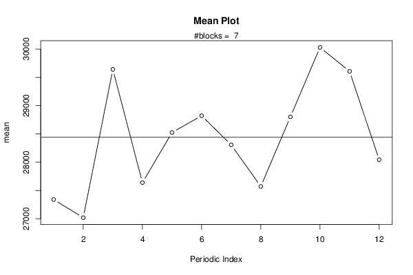
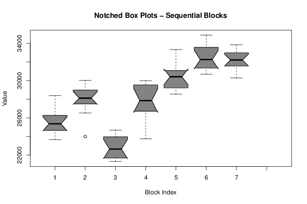
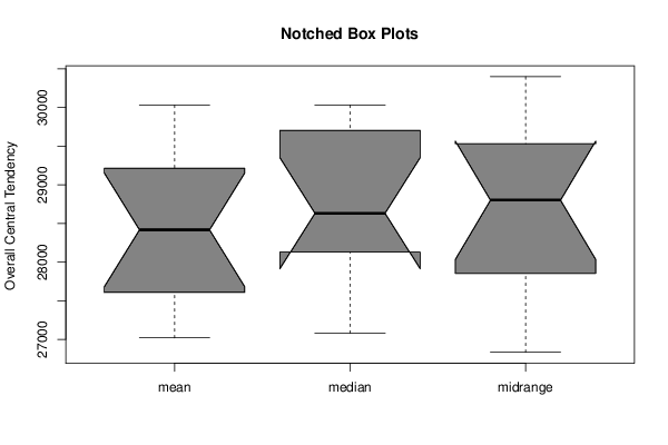
| Title produced by software | Mean Plot | ||||||||||||||||||||
| Date of computation | Thu, 16 Oct 2014 14:06:47 +0100 | ||||||||||||||||||||
| Cite this page as follows | Statistical Computations at FreeStatistics.org, Office for Research Development and Education, URL https://freestatistics.org/blog/index.php?v=date/2014/Oct/16/t1413464877udk7klmsessz610.htm/, Retrieved Mon, 13 May 2024 00:40:34 +0000 | ||||||||||||||||||||
| Statistical Computations at FreeStatistics.org, Office for Research Development and Education, URL https://freestatistics.org/blog/index.php?pk=242358, Retrieved Mon, 13 May 2024 00:40:34 +0000 | |||||||||||||||||||||
| QR Codes: | |||||||||||||||||||||
|
| |||||||||||||||||||||
| Original text written by user: | |||||||||||||||||||||
| IsPrivate? | No (this computation is public) | ||||||||||||||||||||
| User-defined keywords | |||||||||||||||||||||
| Estimated Impact | 92 | ||||||||||||||||||||
Tree of Dependent Computations | |||||||||||||||||||||
| Family? (F = Feedback message, R = changed R code, M = changed R Module, P = changed Parameters, D = changed Data) | |||||||||||||||||||||
| - [Mean Plot] [] [2014-10-10 11:30:26] [646b2e45c853a5eeaa778aa28018f97d] - [Mean Plot] [] [2014-10-16 13:06:47] [e9c24c4a54e855481a8eaf4353236c0f] [Current] - R D [Mean Plot] [] [2014-12-29 09:29:56] [e39bbdb9244073fc72a45a9289b4fb1d] | |||||||||||||||||||||
| Feedback Forum | |||||||||||||||||||||
Post a new message | |||||||||||||||||||||
Dataset | |||||||||||||||||||||
| Dataseries X: | |||||||||||||||||||||
24175 23658 26727 24397 25829 25503 24914 24875 25461 27647 28382 25259 28100 27900 28078 28479 28156 29219 28782 27078 30031 29579 26532 23995 22067 21818 23787 21551 21309 22395 22906 21430 23492 24144 24438 24689 24569 23754 28473 27051 27081 29635 27715 26373 28009 29472 30005 29777 28886 28549 33348 29017 30924 30435 29431 30290 31286 30622 31742 30391 30740 32086 33947 31312 33239 32362 32170 32665 31412 34891 33919 30706 32846 31368 33130 31665 33139 32201 32230 30287 31918 33853 32232 31484 | |||||||||||||||||||||
Tables (Output of Computation) | |||||||||||||||||||||
| |||||||||||||||||||||
Figures (Output of Computation) | |||||||||||||||||||||
Input Parameters & R Code | |||||||||||||||||||||
| Parameters (Session): | |||||||||||||||||||||
| par1 = 12 ; | |||||||||||||||||||||
| Parameters (R input): | |||||||||||||||||||||
| par1 = 12 ; | |||||||||||||||||||||
| R code (references can be found in the software module): | |||||||||||||||||||||
par1 <- as.numeric(par1) | |||||||||||||||||||||