Free Statistics
of Irreproducible Research!
Description of Statistical Computation | |||||||||||||||||||||
|---|---|---|---|---|---|---|---|---|---|---|---|---|---|---|---|---|---|---|---|---|---|
| Author's title | |||||||||||||||||||||
| Author | *Unverified author* | ||||||||||||||||||||
| R Software Module | rwasp_meanplot.wasp | ||||||||||||||||||||
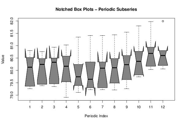
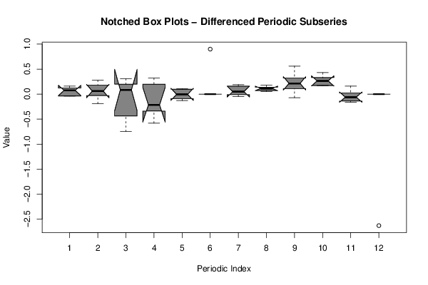
| Title produced by software | Mean Plot | ||||||||||||||||||||
| Date of computation | Mon, 13 Oct 2014 15:48:33 +0100 | ||||||||||||||||||||
| Cite this page as follows | Statistical Computations at FreeStatistics.org, Office for Research Development and Education, URL https://freestatistics.org/blog/index.php?v=date/2014/Oct/13/t1413211864r346z2s2qwt0ktn.htm/, Retrieved Fri, 10 May 2024 09:50:15 +0000 | ||||||||||||||||||||
| Statistical Computations at FreeStatistics.org, Office for Research Development and Education, URL https://freestatistics.org/blog/index.php?pk=240770, Retrieved Fri, 10 May 2024 09:50:15 +0000 | |||||||||||||||||||||
| QR Codes: | |||||||||||||||||||||
|
| |||||||||||||||||||||
| Original text written by user: | |||||||||||||||||||||
| IsPrivate? | No (this computation is public) | ||||||||||||||||||||
| User-defined keywords | |||||||||||||||||||||
| Estimated Impact | 63 | ||||||||||||||||||||
Tree of Dependent Computations | |||||||||||||||||||||
| Family? (F = Feedback message, R = changed R code, M = changed R Module, P = changed Parameters, D = changed Data) | |||||||||||||||||||||
| - [Mean Plot] [] [2014-10-13 14:48:33] [81bcec4b91879990466572cf43afb80d] [Current] | |||||||||||||||||||||
| Feedback Forum | |||||||||||||||||||||
Post a new message | |||||||||||||||||||||
Dataset | |||||||||||||||||||||
| Dataseries X: | |||||||||||||||||||||
79,26 79,38 79,35 78,91 79,11 79,22 79,22 79,21 79,26 79,82 80,04 80,2 80,2 80,27 80,37 80,57 79,99 79,86 79,86 79,81 79,88 80,2 80,53 80,52 80,52 80,48 80,29 79,54 79,39 79,3 79,3 79,49 79,63 79,74 80,17 80,06 80,06 80,22 80,5 80,58 80,24 80,34 80,34 80,41 80,59 80,77 80,94 80,8 80,8 80,76 80,94 81,03 81,35 81,41 81,41 81,44 81,55 81,8 81,97 81,99 79,36 79,44 79,46 79,77 79,49 79,42 80,32 80,48 80,6 80,53 80,84 80,68 | |||||||||||||||||||||
Tables (Output of Computation) | |||||||||||||||||||||
| |||||||||||||||||||||
Figures (Output of Computation) | |||||||||||||||||||||
Input Parameters & R Code | |||||||||||||||||||||
| Parameters (Session): | |||||||||||||||||||||
| par1 = 12 ; | |||||||||||||||||||||
| Parameters (R input): | |||||||||||||||||||||
| par1 = 12 ; | |||||||||||||||||||||
| R code (references can be found in the software module): | |||||||||||||||||||||
par1 <- as.numeric(par1) | |||||||||||||||||||||