Free Statistics
of Irreproducible Research!
Description of Statistical Computation | |||||||||||||||||||||
|---|---|---|---|---|---|---|---|---|---|---|---|---|---|---|---|---|---|---|---|---|---|
| Author's title | |||||||||||||||||||||
| Author | *Unverified author* | ||||||||||||||||||||
| R Software Module | rwasp_sdplot.wasp | ||||||||||||||||||||
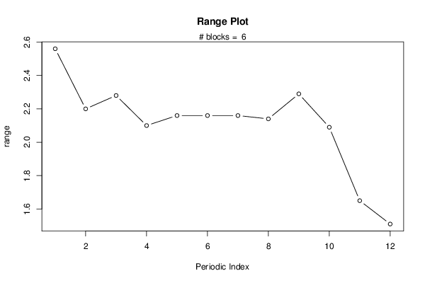
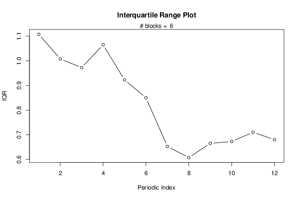
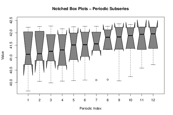
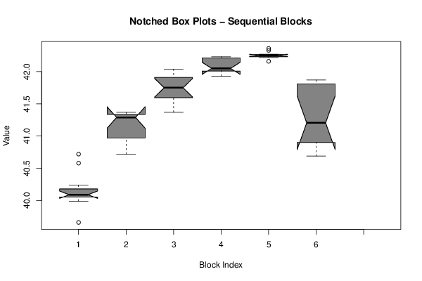
| Title produced by software | Standard Deviation Plot | ||||||||||||||||||||
| Date of computation | Thu, 20 Nov 2014 15:41:36 +0000 | ||||||||||||||||||||
| Cite this page as follows | Statistical Computations at FreeStatistics.org, Office for Research Development and Education, URL https://freestatistics.org/blog/index.php?v=date/2014/Nov/20/t141649812188szkxbp7bxy350.htm/, Retrieved Sun, 19 May 2024 14:40:40 +0000 | ||||||||||||||||||||
| Statistical Computations at FreeStatistics.org, Office for Research Development and Education, URL https://freestatistics.org/blog/index.php?pk=257207, Retrieved Sun, 19 May 2024 14:40:40 +0000 | |||||||||||||||||||||
| QR Codes: | |||||||||||||||||||||
|
| |||||||||||||||||||||
| Original text written by user: | |||||||||||||||||||||
| IsPrivate? | No (this computation is public) | ||||||||||||||||||||
| User-defined keywords | |||||||||||||||||||||
| Estimated Impact | 60 | ||||||||||||||||||||
Tree of Dependent Computations | |||||||||||||||||||||
| Family? (F = Feedback message, R = changed R code, M = changed R Module, P = changed Parameters, D = changed Data) | |||||||||||||||||||||
| - [Standard Deviation Plot] [SD-MP_2_opd9] [2014-11-20 15:41:36] [d0f5aeb11a4aa291a6c63b9267d14d48] [Current] | |||||||||||||||||||||
| Feedback Forum | |||||||||||||||||||||
Post a new message | |||||||||||||||||||||
Dataset | |||||||||||||||||||||
| Dataseries X: | |||||||||||||||||||||
39,66 40,05 39,99 40,06 40,08 40,1 40,1 40,12 40,07 40,24 40,58 40,72 40,72 40,89 40,9 41,04 41,27 41,29 41,29 41,33 41,34 41,37 41,33 41,37 41,37 41,42 41,61 41,58 41,75 41,75 41,75 41,85 41,84 41,97 42,01 42,04 42,04 42,06 41,93 41,93 41,99 42,03 42,03 42,12 42,22 42,21 42,23 42,22 42,22 42,25 42,27 42,16 42,24 42,26 42,26 42,26 42,36 42,33 42,23 42,23 40,9 40,9 40,87 40,69 40,92 41,05 41,36 41,79 41,82 41,8 41,87 41,87 | |||||||||||||||||||||
Tables (Output of Computation) | |||||||||||||||||||||
| |||||||||||||||||||||
Figures (Output of Computation) | |||||||||||||||||||||
Input Parameters & R Code | |||||||||||||||||||||
| Parameters (Session): | |||||||||||||||||||||
| par1 = 12 ; | |||||||||||||||||||||
| Parameters (R input): | |||||||||||||||||||||
| par1 = 12 ; | |||||||||||||||||||||
| R code (references can be found in the software module): | |||||||||||||||||||||
par1 <- as.numeric(par1) | |||||||||||||||||||||