Free Statistics
of Irreproducible Research!
Description of Statistical Computation | ||||||||||||||||||||||||||||||
|---|---|---|---|---|---|---|---|---|---|---|---|---|---|---|---|---|---|---|---|---|---|---|---|---|---|---|---|---|---|---|
| Author's title | ||||||||||||||||||||||||||||||
| Author | *The author of this computation has been verified* | |||||||||||||||||||||||||||||
| R Software Module | rwasp_Distributional Plots.wasp | |||||||||||||||||||||||||||||
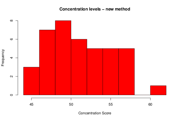
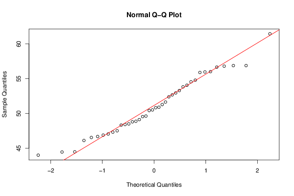
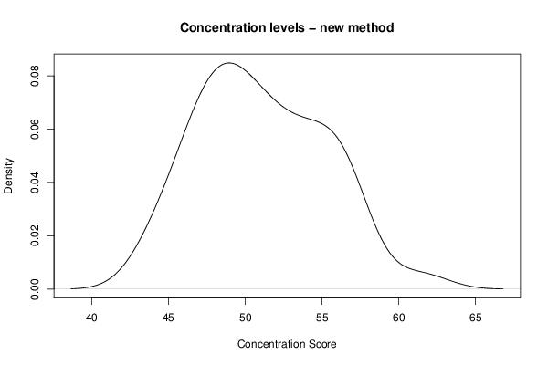
| Title produced by software | Histogram, QQplot and Density | |||||||||||||||||||||||||||||
| Date of computation | Thu, 06 Nov 2014 14:27:35 +0000 | |||||||||||||||||||||||||||||
| Cite this page as follows | Statistical Computations at FreeStatistics.org, Office for Research Development and Education, URL https://freestatistics.org/blog/index.php?v=date/2014/Nov/06/t1415284066a4vasjf8k7qd5ci.htm/, Retrieved Sun, 19 May 2024 14:07:08 +0000 | |||||||||||||||||||||||||||||
| Statistical Computations at FreeStatistics.org, Office for Research Development and Education, URL https://freestatistics.org/blog/index.php?pk=252692, Retrieved Sun, 19 May 2024 14:07:08 +0000 | ||||||||||||||||||||||||||||||
| QR Codes: | ||||||||||||||||||||||||||||||
|
| ||||||||||||||||||||||||||||||
| Original text written by user: | ||||||||||||||||||||||||||||||
| IsPrivate? | No (this computation is public) | |||||||||||||||||||||||||||||
| User-defined keywords | ||||||||||||||||||||||||||||||
| Estimated Impact | 37 | |||||||||||||||||||||||||||||
Tree of Dependent Computations | ||||||||||||||||||||||||||||||
| Family? (F = Feedback message, R = changed R code, M = changed R Module, P = changed Parameters, D = changed Data) | ||||||||||||||||||||||||||||||
| - [Aston University Statistical Software] [Morning Sickness ...] [2009-11-16 16:26:06] [74be16979710d4c4e7c6647856088456] - R [Aston University Statistical Software] [Morning Sickness ...] [2009-11-16 17:22:16] [74be16979710d4c4e7c6647856088456] - P [T-Tests] [Morning Sickness ...] [2010-11-09 11:12:43] [3fdd735c61ad38cbc9b3393dc997cdb7] - RM [T-Tests] [Morning Sickness ...] [2011-11-07 09:34:35] [98fd0e87c3eb04e0cc2efde01dbafab6] - RMPD [Histogram, QQplot and Density] [blog8] [2014-11-06 14:27:35] [5bfcbb8e4e9d59dd95833827525d5e53] [Current] | ||||||||||||||||||||||||||||||
| Feedback Forum | ||||||||||||||||||||||||||||||
Post a new message | ||||||||||||||||||||||||||||||
Dataset | ||||||||||||||||||||||||||||||
| Dataseries X: | ||||||||||||||||||||||||||||||
46.12 50.9 47.32 47.05 49.55 48.33 44.49 51.64 46.55 54.79 47.51 50.83 48.41 53.83 52.95 56.88 48.5 53.29 54.06 56.66 48.88 44.46 49.63 49.12 56.88 46.89 55.97 50.42 52.67 51.28 55.89 54.55 48.8 52.39 56.8 46.69 44.01 50.51 56.01 61.45 | ||||||||||||||||||||||||||||||
Tables (Output of Computation) | ||||||||||||||||||||||||||||||
| ||||||||||||||||||||||||||||||
Figures (Output of Computation) | ||||||||||||||||||||||||||||||
Input Parameters & R Code | ||||||||||||||||||||||||||||||
| Parameters (Session): | ||||||||||||||||||||||||||||||
| par1 = 10 ; | ||||||||||||||||||||||||||||||
| Parameters (R input): | ||||||||||||||||||||||||||||||
| par1 = 10 ; | ||||||||||||||||||||||||||||||
| R code (references can be found in the software module): | ||||||||||||||||||||||||||||||
x <- x[!is.na(x)] | ||||||||||||||||||||||||||||||