Free Statistics
of Irreproducible Research!
Description of Statistical Computation | |||||||||||||||||||||||||||||||||||||||||||||||||||||||||||||||||||||||||||||||||||||||||||||||||||||||||||||||||||||||||||||||||||||||||||||||||||||||||||||||||
|---|---|---|---|---|---|---|---|---|---|---|---|---|---|---|---|---|---|---|---|---|---|---|---|---|---|---|---|---|---|---|---|---|---|---|---|---|---|---|---|---|---|---|---|---|---|---|---|---|---|---|---|---|---|---|---|---|---|---|---|---|---|---|---|---|---|---|---|---|---|---|---|---|---|---|---|---|---|---|---|---|---|---|---|---|---|---|---|---|---|---|---|---|---|---|---|---|---|---|---|---|---|---|---|---|---|---|---|---|---|---|---|---|---|---|---|---|---|---|---|---|---|---|---|---|---|---|---|---|---|---|---|---|---|---|---|---|---|---|---|---|---|---|---|---|---|---|---|---|---|---|---|---|---|---|---|---|---|---|---|---|---|
| Author's title | |||||||||||||||||||||||||||||||||||||||||||||||||||||||||||||||||||||||||||||||||||||||||||||||||||||||||||||||||||||||||||||||||||||||||||||||||||||||||||||||||
| Author | *The author of this computation has been verified* | ||||||||||||||||||||||||||||||||||||||||||||||||||||||||||||||||||||||||||||||||||||||||||||||||||||||||||||||||||||||||||||||||||||||||||||||||||||||||||||||||
| R Software Module | rwasp_bootstrapplot1.wasp | ||||||||||||||||||||||||||||||||||||||||||||||||||||||||||||||||||||||||||||||||||||||||||||||||||||||||||||||||||||||||||||||||||||||||||||||||||||||||||||||||
| Title produced by software | Bootstrap Plot - Central Tendency | ||||||||||||||||||||||||||||||||||||||||||||||||||||||||||||||||||||||||||||||||||||||||||||||||||||||||||||||||||||||||||||||||||||||||||||||||||||||||||||||||
| Date of computation | Tue, 04 Nov 2014 10:49:59 +0000 | ||||||||||||||||||||||||||||||||||||||||||||||||||||||||||||||||||||||||||||||||||||||||||||||||||||||||||||||||||||||||||||||||||||||||||||||||||||||||||||||||
| Cite this page as follows | Statistical Computations at FreeStatistics.org, Office for Research Development and Education, URL https://freestatistics.org/blog/index.php?v=date/2014/Nov/04/t1415098273nldx4us1u0f1hjd.htm/, Retrieved Sun, 19 May 2024 17:14:55 +0000 | ||||||||||||||||||||||||||||||||||||||||||||||||||||||||||||||||||||||||||||||||||||||||||||||||||||||||||||||||||||||||||||||||||||||||||||||||||||||||||||||||
| Statistical Computations at FreeStatistics.org, Office for Research Development and Education, URL https://freestatistics.org/blog/index.php?pk=251183, Retrieved Sun, 19 May 2024 17:14:55 +0000 | |||||||||||||||||||||||||||||||||||||||||||||||||||||||||||||||||||||||||||||||||||||||||||||||||||||||||||||||||||||||||||||||||||||||||||||||||||||||||||||||||
| QR Codes: | |||||||||||||||||||||||||||||||||||||||||||||||||||||||||||||||||||||||||||||||||||||||||||||||||||||||||||||||||||||||||||||||||||||||||||||||||||||||||||||||||
|
| |||||||||||||||||||||||||||||||||||||||||||||||||||||||||||||||||||||||||||||||||||||||||||||||||||||||||||||||||||||||||||||||||||||||||||||||||||||||||||||||||
| Original text written by user: | |||||||||||||||||||||||||||||||||||||||||||||||||||||||||||||||||||||||||||||||||||||||||||||||||||||||||||||||||||||||||||||||||||||||||||||||||||||||||||||||||
| IsPrivate? | No (this computation is public) | ||||||||||||||||||||||||||||||||||||||||||||||||||||||||||||||||||||||||||||||||||||||||||||||||||||||||||||||||||||||||||||||||||||||||||||||||||||||||||||||||
| User-defined keywords | |||||||||||||||||||||||||||||||||||||||||||||||||||||||||||||||||||||||||||||||||||||||||||||||||||||||||||||||||||||||||||||||||||||||||||||||||||||||||||||||||
| Estimated Impact | 367 | ||||||||||||||||||||||||||||||||||||||||||||||||||||||||||||||||||||||||||||||||||||||||||||||||||||||||||||||||||||||||||||||||||||||||||||||||||||||||||||||||
Tree of Dependent Computations | |||||||||||||||||||||||||||||||||||||||||||||||||||||||||||||||||||||||||||||||||||||||||||||||||||||||||||||||||||||||||||||||||||||||||||||||||||||||||||||||||
| Family? (F = Feedback message, R = changed R code, M = changed R Module, P = changed Parameters, D = changed Data) | |||||||||||||||||||||||||||||||||||||||||||||||||||||||||||||||||||||||||||||||||||||||||||||||||||||||||||||||||||||||||||||||||||||||||||||||||||||||||||||||||
| - [Bootstrap Plot - Central Tendency] [] [2014-11-04 10:49:59] [63a9f0ea7bb98050796b649e85481845] [Current] - D [Bootstrap Plot - Central Tendency] [] [2014-11-06 19:33:20] [8f0f7d8870e334acea674e48ede2c797] - R D [Bootstrap Plot - Central Tendency] [WS7] [2014-11-08 09:49:52] [877240ca1fa14bdfceaf44d965b0fbd7] - R D [Bootstrap Plot - Central Tendency] [] [2014-11-11 18:42:11] [67894a4ff6098ffac356bc81e6028257] - R D [Bootstrap Plot - Central Tendency] [] [2014-11-11 18:47:44] [67894a4ff6098ffac356bc81e6028257] - R [Bootstrap Plot - Central Tendency] [WS7 task3] [2014-11-12 08:30:35] [46c7ebd23dbdec306a09830d8b7528e7] - R D [Bootstrap Plot - Central Tendency] [Depression model ...] [2014-11-12 13:28:42] [81f624c2f0b20a2549c93e7c3dccf981] - RM [Bootstrap Plot - Central Tendency] [] [2014-11-12 13:47:16] [1e6e0879de81abfeb504403e705bc72d] - R [Bootstrap Plot - Central Tendency] [] [2014-11-12 13:49:48] [1e6e0879de81abfeb504403e705bc72d] - RM [Bootstrap Plot - Central Tendency] [ws7 v3] [2014-11-12 13:52:03] [e3727f74ca0896859afbe865e40a3465] - R D [Bootstrap Plot - Central Tendency] [] [2014-11-12 13:54:32] [6795cd14e59cd8fafcdf800c40b889d9] - RM [Bootstrap Plot - Central Tendency] [] [2014-11-12 13:57:35] [93cb0d178904cf975da218b7c929e42d] - RM [Bootstrap Plot - Central Tendency] [] [2014-11-12 13:57:46] [eee95947b6243a1febfcd5f41483d733] - RM [Bootstrap Plot - Central Tendency] [] [2014-11-12 14:31:51] [b2fe7fef0850359c2a41ad606a8f04c2] - R [Bootstrap Plot - Central Tendency] [] [2014-11-12 14:40:45] [c2c160edf30e228bd3a949bf24376c2c] - R [Bootstrap Plot - Central Tendency] [WS 7: bootstrap] [2014-11-12 14:42:48] [36781f05c04c55e165b348994b753b95] - R [Bootstrap Plot - Central Tendency] [] [2014-11-12 14:44:09] [c2c160edf30e228bd3a949bf24376c2c] - R [Bootstrap Plot - Central Tendency] [WS 7: bootstrap] [2014-11-12 14:45:14] [36781f05c04c55e165b348994b753b95] - R [Bootstrap Plot - Central Tendency] [] [2014-11-12 15:10:15] [dacad244957cb51472792888970d4390] - R [Bootstrap Plot - Central Tendency] [WS7 Q3] [2014-11-12 15:25:03] [bcf5edf18529a33bd1494456d2c6cb9a] - R D [Bootstrap Plot - Central Tendency] [] [2014-11-12 15:33:27] [d253a55552bf9917a397def3be261e30] - D [Bootstrap Plot - Central Tendency] [] [2014-12-13 12:30:20] [d253a55552bf9917a397def3be261e30] - D [Bootstrap Plot - Central Tendency] [] [2014-12-14 13:00:35] [d253a55552bf9917a397def3be261e30] - R [Bootstrap Plot - Central Tendency] [WS7 SHW] [2014-11-12 15:36:39] [cac6c5fb035463be46c296b46e439cb5] - RM [Bootstrap Plot - Central Tendency] [WS7 Q4] [2014-11-12 15:37:27] [bcf5edf18529a33bd1494456d2c6cb9a] - RM [Bootstrap Plot - Central Tendency] [] [2014-11-12 15:48:49] [3cc57788b191749bdc089f5fad42e0f8] - RM [Bootstrap Plot - Central Tendency] [] [2014-11-12 16:22:56] [d253a55552bf9917a397def3be261e30] - RM [Bootstrap Plot - Central Tendency] [] [2014-11-12 16:28:30] [d253a55552bf9917a397def3be261e30] - RM D [Bootstrap Plot - Central Tendency] [] [2014-12-16 12:54:33] [d253a55552bf9917a397def3be261e30] - R [Bootstrap Plot - Central Tendency] [] [2014-11-12 16:34:11] [6656361aa4da5489a6a45e803df0211c] - R [Bootstrap Plot - Central Tendency] [] [2014-11-12 16:35:36] [6656361aa4da5489a6a45e803df0211c] - RM [Bootstrap Plot - Central Tendency] [] [2014-11-12 16:52:03] [261f60062b6e70d0e3f72a6ad4f04654] - [Bootstrap Plot - Central Tendency] [] [2014-11-12 17:04:49] [bca3c6529212edfac3e771806c79a908] - P [Bootstrap Plot - Central Tendency] [] [2014-11-12 18:12:10] [9bd698ecfffbb3f270ebcac6c258c074] - R D [Bootstrap Plot - Central Tendency] [mean] [2014-11-12 18:13:55] [3d5212c89039da1a3a24d8e18d23c716] - R [Bootstrap Plot - Central Tendency] [bootstrap plot] [2014-11-12 18:42:56] [1e921ed6280e31020168fe5cd3fc7265] - RM [Bootstrap Plot - Central Tendency] [WS7 - 3] [2014-11-12 19:07:49] [4d39cf209776852399955073f9d0ee7a] - [Bootstrap Plot - Central Tendency] [WSH 7, 6] [2014-11-13 19:29:00] [e7da31d1eb6eab8d5ed70d87d07c747b] - [Bootstrap Plot - Central Tendency] [WSH 7, 7] [2014-11-13 19:30:22] [e7da31d1eb6eab8d5ed70d87d07c747b] - [Bootstrap Plot - Central Tendency] [WSH 7, 8] [2014-11-13 19:31:59] [e7da31d1eb6eab8d5ed70d87d07c747b] - [Bootstrap Plot - Central Tendency] [WSH 7, 9] [2014-11-13 19:33:29] [e7da31d1eb6eab8d5ed70d87d07c747b] - R [Bootstrap Plot - Central Tendency] [] [2014-11-12 20:56:25] [99723d3e379f668157309b7b2091b15d] - R [Bootstrap Plot - Central Tendency] [qsdqsd] [2014-11-13 13:22:53] [9378e2688aa9dcfd1390615d31e9d404] - RM [Bootstrap Plot - Central Tendency] [] [2014-11-13 13:27:06] [dd7a37d66cc3f8699a204e53c0324369] - R [Bootstrap Plot - Central Tendency] [] [2014-11-13 18:20:46] [02fb6cbf799bcf1e525e4e01c2f27ada] - R D [Bootstrap Plot - Central Tendency] [ws7] [2014-11-13 18:27:03] [8523551e1e4e3cbe97fa25692e177b2e] - RM [Bootstrap Plot - Central Tendency] [q] [2014-11-13 18:53:37] [1651e47f7f65f3a10bbbb444d4b26be7] - R D [Bootstrap Plot - Central Tendency] [] [2014-11-13 20:13:25] [fda96889f4ef6d31c0c28fd64d281011] - RM [Bootstrap Plot - Central Tendency] [sim med] [2014-11-13 20:38:14] [4987e1e3573a375c88e9a0c129fd9e05] [Truncated] | |||||||||||||||||||||||||||||||||||||||||||||||||||||||||||||||||||||||||||||||||||||||||||||||||||||||||||||||||||||||||||||||||||||||||||||||||||||||||||||||||
| Feedback Forum | |||||||||||||||||||||||||||||||||||||||||||||||||||||||||||||||||||||||||||||||||||||||||||||||||||||||||||||||||||||||||||||||||||||||||||||||||||||||||||||||||
Post a new message | |||||||||||||||||||||||||||||||||||||||||||||||||||||||||||||||||||||||||||||||||||||||||||||||||||||||||||||||||||||||||||||||||||||||||||||||||||||||||||||||||
Dataset | |||||||||||||||||||||||||||||||||||||||||||||||||||||||||||||||||||||||||||||||||||||||||||||||||||||||||||||||||||||||||||||||||||||||||||||||||||||||||||||||||
| Dataseries X: | |||||||||||||||||||||||||||||||||||||||||||||||||||||||||||||||||||||||||||||||||||||||||||||||||||||||||||||||||||||||||||||||||||||||||||||||||||||||||||||||||
0.294153 2.97156 -2.71955 -2.10608 5.15598 3.88145 3.48012 -0.793748 0.0474647 0.949459 1.70415 3.53959 -3.16424 2.70588 2.45478 0.885167 0.432262 1.36526 -1.255 2.42932 2.88737 -2.42299 -0.36997 -1.32201 1.79733 -6.83795 1.13673 0.968342 1.29799 -2.62899 0.532419 0.742768 2.12812 -0.0241935 0.256096 0.854528 -1.36766 0.889595 1.90098 -2.04375 -0.553176 2.57853 0.103225 -0.921825 0.567044 -2.36129 -0.183641 0.333117 3.66465 -1.59683 0.909003 0.806532 -0.386175 -1.39188 -1.72474 1.63465 1.91825 -0.283804 -3.07451 -1.19565 -2.36197 -1.51284 -3.52005 1.12206 1.48021 -5.05159 -1.57071 -2.46861 1.56108 1.43552 0.719528 3.42149 0.566379 -0.363746 -1.9214 -0.056789 3.01548 0.632589 1.37487 -2.02638 0.115316 -0.491874 1.71652 0.792612 -0.0500028 1.06084 -0.257791 0.293489 -3.39489 3.46282 0.104144 0.834079 0.760705 -0.886211 0.991821 -0.812128 -0.861605 2.03306 0.0326958 1.75233 -0.919433 0.872158 -3.38395 1.95822 -2.34112 1.01075 2.0363 -2.8444 0.975645 1.16927 -2.19003 -2.24943 1.93964 3.96052 0.344235 1.01153 0.283773 -1.06596 0.296354 -0.483775 0.441724 0.121994 -1.00658 0.382647 -1.80252 0.786913 1.54651 4.15924 1.47515 -1.67088 -1.41748 -0.355202 2.53319 0.754977 2.30513 1.73636 0.713535 -0.826256 0.873435 -0.698291 0.318378 2.25138 -0.706501 0.692002 1.48385 1.44925 -2.39905 -2.72706 -2.40806 1.89067 0.355387 0.489124 -2.45246 -2.4997 1.47025 0.104144 0.770858 4.15924 -2.73299 0.0487413 0.520571 0.817289 0.750211 4.29504 -2.03717 2.04186 -0.19388 -0.864039 -3.7685 -3.03779 0.446489 1.59975 -5.15257 1.75479 2.51998 -2.48453 -3.35533 0.512109 1.30535 -2.29359 -0.352145 -1.80944 0.0351127 -1.20099 2.02659 1.20875 0.216629 0.686974 0.498628 0.817199 -1.94897 -1.28106 2.27819 -1.65853 1.7838 -2.26586 2.1398 0.426097 -3.24974 -0.945592 -3.29269 1.12158 2.78591 0.297647 0.379211 1.07392 -0.692765 3.21317 -0.0115483 1.49078 -2.81386 1.25588 -1.34621 -3.96611 -1.36908 1.58447 1.86706 -0.45464 -2.05585 1.21455 -3.09837 2.11414 -2.31201 0.0218416 -0.877228 1.63328 4.97042 -1.91696 -1.51227 -2.50048 0.0158494 -3.08591 -0.165203 0.240808 0.874019 -1.99099 0.755342 -0.0764699 -4.61544 -2.70354 -2.92081 -2.85065 0.241454 -0.409056 1.2673 0.219823 0.100763 5.08859 -0.195174 0.358255 2.02625 1.07606 -1.31709 -0.952895 0.0362316 -0.868792 -2.06858 -2.59497 2.19119 -4.78671 0.0887831 1.2742 -2.92786 -0.0466467 | |||||||||||||||||||||||||||||||||||||||||||||||||||||||||||||||||||||||||||||||||||||||||||||||||||||||||||||||||||||||||||||||||||||||||||||||||||||||||||||||||
Tables (Output of Computation) | |||||||||||||||||||||||||||||||||||||||||||||||||||||||||||||||||||||||||||||||||||||||||||||||||||||||||||||||||||||||||||||||||||||||||||||||||||||||||||||||||
| |||||||||||||||||||||||||||||||||||||||||||||||||||||||||||||||||||||||||||||||||||||||||||||||||||||||||||||||||||||||||||||||||||||||||||||||||||||||||||||||||
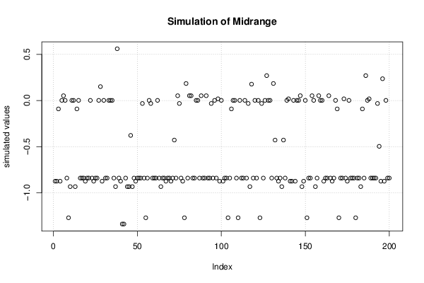
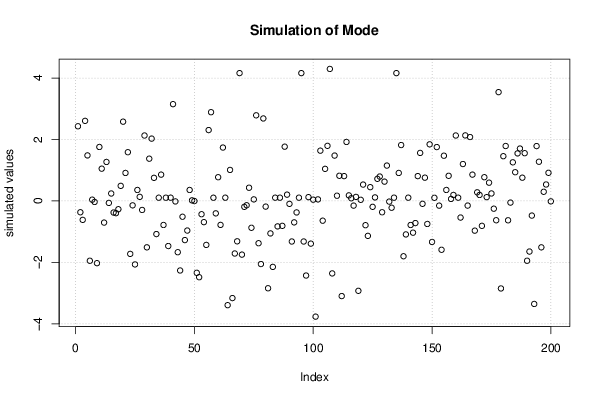
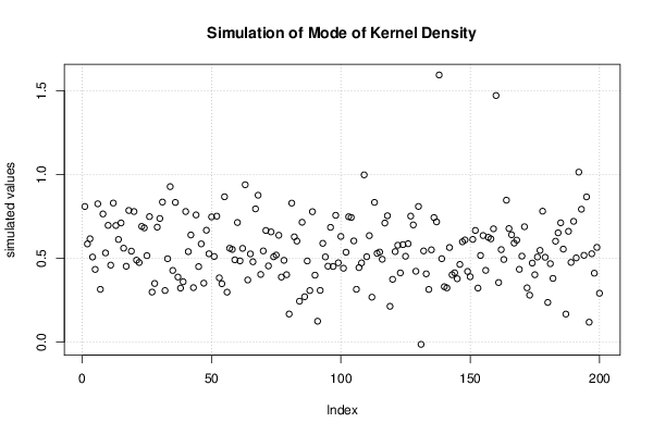
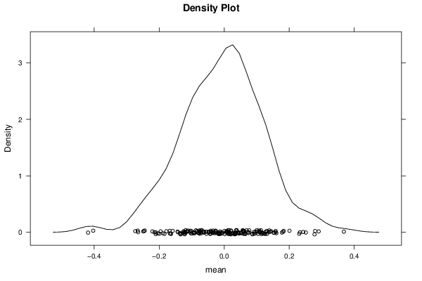
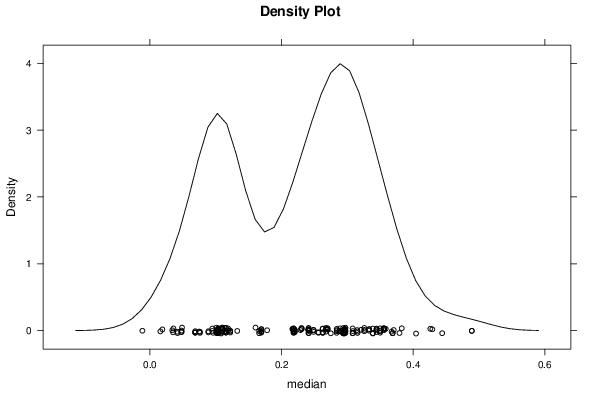
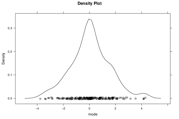
Figures (Output of Computation) | |||||||||||||||||||||||||||||||||||||||||||||||||||||||||||||||||||||||||||||||||||||||||||||||||||||||||||||||||||||||||||||||||||||||||||||||||||||||||||||||||
Input Parameters & R Code | |||||||||||||||||||||||||||||||||||||||||||||||||||||||||||||||||||||||||||||||||||||||||||||||||||||||||||||||||||||||||||||||||||||||||||||||||||||||||||||||||
| Parameters (Session): | |||||||||||||||||||||||||||||||||||||||||||||||||||||||||||||||||||||||||||||||||||||||||||||||||||||||||||||||||||||||||||||||||||||||||||||||||||||||||||||||||
| par1 = 200 ; par2 = 5 ; par3 = 0 ; par4 = P1 P5 Q1 Q3 P95 P99 ; | |||||||||||||||||||||||||||||||||||||||||||||||||||||||||||||||||||||||||||||||||||||||||||||||||||||||||||||||||||||||||||||||||||||||||||||||||||||||||||||||||
| Parameters (R input): | |||||||||||||||||||||||||||||||||||||||||||||||||||||||||||||||||||||||||||||||||||||||||||||||||||||||||||||||||||||||||||||||||||||||||||||||||||||||||||||||||
| par1 = 200 ; par2 = 5 ; par3 = 0 ; par4 = P1 P5 Q1 Q3 P95 P99 ; | |||||||||||||||||||||||||||||||||||||||||||||||||||||||||||||||||||||||||||||||||||||||||||||||||||||||||||||||||||||||||||||||||||||||||||||||||||||||||||||||||
| R code (references can be found in the software module): | |||||||||||||||||||||||||||||||||||||||||||||||||||||||||||||||||||||||||||||||||||||||||||||||||||||||||||||||||||||||||||||||||||||||||||||||||||||||||||||||||
par1 <- as.numeric(par1) | |||||||||||||||||||||||||||||||||||||||||||||||||||||||||||||||||||||||||||||||||||||||||||||||||||||||||||||||||||||||||||||||||||||||||||||||||||||||||||||||||