Free Statistics
of Irreproducible Research!
Description of Statistical Computation | ||||||||||||||||||||||||||||||
|---|---|---|---|---|---|---|---|---|---|---|---|---|---|---|---|---|---|---|---|---|---|---|---|---|---|---|---|---|---|---|
| Author's title | ||||||||||||||||||||||||||||||
| Author | *The author of this computation has been verified* | |||||||||||||||||||||||||||||
| R Software Module | rwasp_Distributional Plots.wasp | |||||||||||||||||||||||||||||
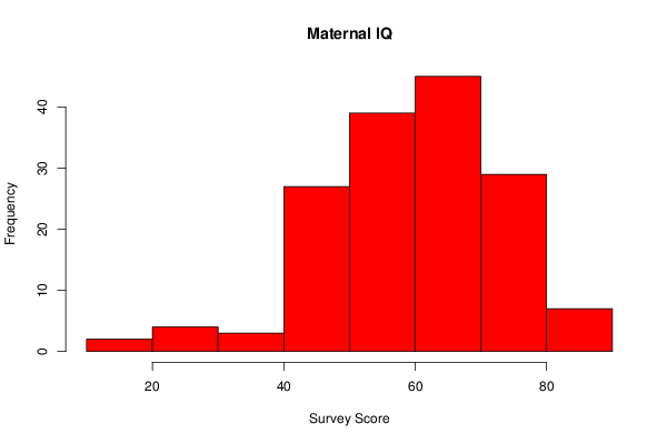
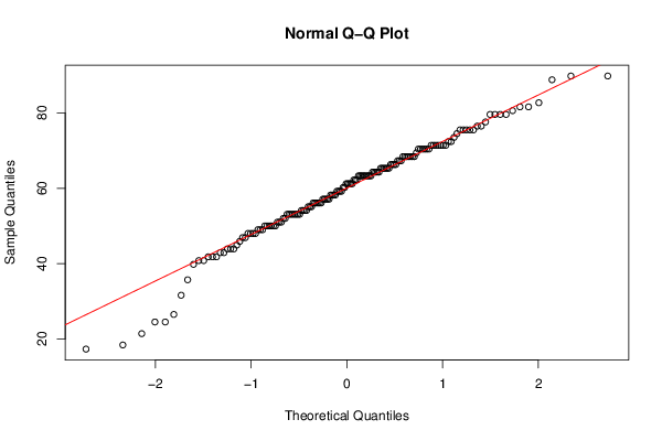
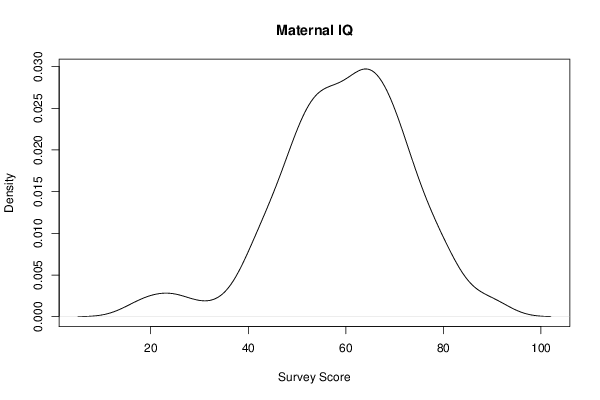
| Title produced by software | Histogram, QQplot and Density | |||||||||||||||||||||||||||||
| Date of computation | Tue, 14 Jan 2014 05:11:46 -0500 | |||||||||||||||||||||||||||||
| Cite this page as follows | Statistical Computations at FreeStatistics.org, Office for Research Development and Education, URL https://freestatistics.org/blog/index.php?v=date/2014/Jan/14/t1389694381whr2c3yqea505vi.htm/, Retrieved Sun, 19 May 2024 10:21:30 +0000 | |||||||||||||||||||||||||||||
| Statistical Computations at FreeStatistics.org, Office for Research Development and Education, URL https://freestatistics.org/blog/index.php?pk=233138, Retrieved Sun, 19 May 2024 10:21:30 +0000 | ||||||||||||||||||||||||||||||
| QR Codes: | ||||||||||||||||||||||||||||||
|
| ||||||||||||||||||||||||||||||
| Original text written by user: | ||||||||||||||||||||||||||||||
| IsPrivate? | No (this computation is public) | |||||||||||||||||||||||||||||
| User-defined keywords | Percent adjusted scores | |||||||||||||||||||||||||||||
| Estimated Impact | 176 | |||||||||||||||||||||||||||||
Tree of Dependent Computations | ||||||||||||||||||||||||||||||
| Family? (F = Feedback message, R = changed R code, M = changed R Module, P = changed Parameters, D = changed Data) | ||||||||||||||||||||||||||||||
| - [Histogram, QQplot and Density] [PY2224 Advanced S...] [2014-01-14 10:11:46] [a9208f4f8d3b118336aae915785f2bd9] [Current] | ||||||||||||||||||||||||||||||
| Feedback Forum | ||||||||||||||||||||||||||||||
Post a new message | ||||||||||||||||||||||||||||||
Dataset | ||||||||||||||||||||||||||||||
| Dataseries X: | ||||||||||||||||||||||||||||||
75.5 71.4 89.8 57.1 67.3 24.5 46.9 58.2 61.2 50.0 63.3 68.4 41.8 50.0 82.7 43.9 75.5 48.0 56.1 61.2 64.3 58.2 65.3 54.1 70.4 65.3 62.2 63.3 66.3 59.2 61.2 62.2 76.5 63.3 50.0 49.0 39.8 76.5 67.3 24.5 68.4 64.3 75.5 70.4 75.5 51.0 63.3 56.1 43.9 71.4 53.1 54.1 67.3 89.8 63.3 58.2 53.1 50.0 63.3 66.3 55.1 57.1 55.1 49.0 73.5 48.0 70.4 53.1 65.3 54.1 54.1 57.1 65.3 81.6 74.5 71.4 44.9 68.4 57.1 65.3 68.4 55.1 53.1 66.3 63.3 46.9 60.2 68.4 71.4 50.0 61.2 81.6 71.4 80.6 42.9 56.1 40.8 77.6 52.0 59.2 45.9 64.3 56.1 88.8 70.4 52.0 35.7 48.0 43.9 79.6 58.2 41.8 79.6 48.0 53.1 53.1 75.5 18.4 51.0 61.2 53.1 66.3 72.4 79.6 51.0 40.8 50.0 63.3 57.1 26.5 49.0 71.4 42.9 69.4 53.1 60.2 41.8 68.4 70.4 56.1 68.4 64.3 70.4 63.3 31.6 72.4 65.3 59.2 21.4 64.3 71.4 62.2 59.2 56.1 79.6 17.3 | ||||||||||||||||||||||||||||||
Tables (Output of Computation) | ||||||||||||||||||||||||||||||
| ||||||||||||||||||||||||||||||
Figures (Output of Computation) | ||||||||||||||||||||||||||||||
Input Parameters & R Code | ||||||||||||||||||||||||||||||
| Parameters (Session): | ||||||||||||||||||||||||||||||
| par1 = 10 ; | ||||||||||||||||||||||||||||||
| Parameters (R input): | ||||||||||||||||||||||||||||||
| par1 = 10 ; | ||||||||||||||||||||||||||||||
| R code (references can be found in the software module): | ||||||||||||||||||||||||||||||
x <- x[!is.na(x)] | ||||||||||||||||||||||||||||||