Free Statistics

of Irreproducible Research!

Author's title

Author*Unverified author*
R Software Modulerwasp_centraltendency.wasp
Title produced by softwareCentral Tendency
Date of computationSat, 11 Jan 2014 07:57:57 -0500
Cite this page as followsStatistical Computations at FreeStatistics.org, Office for Research Development and Education, URL https://freestatistics.org/blog/index.php?v=date/2014/Jan/11/t1389445207qfjwenuh6xzuk6q.htm/, Retrieved Sun, 19 May 2024 11:33:20 +0000
Statistical Computations at FreeStatistics.org, Office for Research Development and Education, URL https://freestatistics.org/blog/index.php?pk=232899, Retrieved Sun, 19 May 2024 11:33:20 +0000
QR Codes:

Original text written by user:
IsPrivate?No (this computation is public)
User-defined keywords
Estimated Impact157
Family? (F = Feedback message, R = changed R code, M = changed R Module, P = changed Parameters, D = changed Data)
-     [Mean versus Median] [Maximumprijs Show...] [2011-10-16 22:30:32] [102faec22d2a25d9aaa52ca244269a51]
- RM D    [Central Tendency] [] [2014-01-11 12:57:57] [62a6597007cd6653b71a687b26797f80] [Current]
- RM D      [Mean versus Median] [] [2014-01-11 13:08:01] [69f0adfa1a431ec50764c1a969b4d177]
- RMPD      [Univariate Data Series] [] [2014-01-11 14:01:21] [69f0adfa1a431ec50764c1a969b4d177]
- RMPD      [Mean Plot] [] [2014-01-11 14:06:10] [69f0adfa1a431ec50764c1a969b4d177]
- RMP       [Mean Plot] [] [2014-01-11 14:38:19] [69f0adfa1a431ec50764c1a969b4d177]
- RMPD        [(Partial) Autocorrelation Function] [] [2014-01-11 15:29:33] [69f0adfa1a431ec50764c1a969b4d177]
- RMPD        [(Partial) Autocorrelation Function] [] [2014-01-11 15:48:39] [69f0adfa1a431ec50764c1a969b4d177]
- RMP         [(Partial) Autocorrelation Function] [] [2014-01-11 15:55:15] [69f0adfa1a431ec50764c1a969b4d177]
- R  D          [(Partial) Autocorrelation Function] [] [2014-01-11 15:56:26] [69f0adfa1a431ec50764c1a969b4d177]
- RM D          [Bootstrap Plot - Central Tendency] [] [2014-01-11 17:23:05] [69f0adfa1a431ec50764c1a969b4d177]
- R               [Bootstrap Plot - Central Tendency] [] [2014-01-11 17:25:16] [69f0adfa1a431ec50764c1a969b4d177]
-                   [Bootstrap Plot - Central Tendency] [] [2014-01-11 17:39:28] [69f0adfa1a431ec50764c1a969b4d177]
Feedback Forum

Post a new message
Dataseries X:
103,43
103,49
103,5
103,5
103,5
103,5
103,54
103,71
103,76
103,76
103,76
103,82
105,11
105,58
105,91
105,92
105,92
105,92
105,96
105,98
105,98
105,98
106,01
106,01
106,91
107,11
107,18
107,2
107,35
107,35
107,35
107,52
107,56
107,55
107,6
107,6
110,04
110,27
110,33
110,33
110,33
110,33
110,33
110,35
110,38
110,54
110,54
110,54
110,54
106,74
106,78
106,75
106,75
106,75
106,82
107,08
107,25
107,28
107,28
107,28
108,44
109,33
109,44
109,44
109,45
109,45
109,45
109,45
109,46
109,46
109,46
109,46
110,95
110,95
110,95
110,95
110,95
110,95
110,95
110,95
110,97
110,97
110,97
111


Summary of computational transaction
Raw Inputview raw input (R code)
Raw Outputview raw output of R engine
Computing time4 seconds
R Server'Gertrude Mary Cox' @ cox.wessa.net

\begin{tabular}{lllllllll}
\hline
Summary of computational transaction \tabularnewline
Raw Input & view raw input (R code)  \tabularnewline
Raw Output & view raw output of R engine  \tabularnewline
Computing time & 4 seconds \tabularnewline
R Server & 'Gertrude Mary Cox' @ cox.wessa.net \tabularnewline
\hline
\end{tabular}
%Source: https://freestatistics.org/blog/index.php?pk=232899&T=0

[TABLE]
[ROW][C]Summary of computational transaction[/C][/ROW]
[ROW][C]Raw Input[/C][C]view raw input (R code) [/C][/ROW]
[ROW][C]Raw Output[/C][C]view raw output of R engine [/C][/ROW]
[ROW][C]Computing time[/C][C]4 seconds[/C][/ROW]
[ROW][C]R Server[/C][C]'Gertrude Mary Cox' @ cox.wessa.net[/C][/ROW]
[/TABLE]
Source: https://freestatistics.org/blog/index.php?pk=232899&T=0

Globally Unique Identifier (entire table): ba.freestatistics.org/blog/index.php?pk=232899&T=0

As an alternative you can also use a QR Code:  

The GUIDs for individual cells are displayed in the table below:

Summary of computational transaction
Raw Inputview raw input (R code)
Raw Outputview raw output of R engine
Computing time4 seconds
R Server'Gertrude Mary Cox' @ cox.wessa.net


Central Tendency - Ungrouped Data
MeasureValueS.E.Value/S.E.
Arithmetic Mean107.8242857142860.268978128607832400.86636884701
Geometric Mean107.796300592325
Harmonic Mean107.76818055587
Quadratic Mean107.852128287718
Winsorized Mean ( 1 / 28 )107.8246428571430.268787861890404401.151458621697
Winsorized Mean ( 2 / 28 )107.8248809523810.268741648874111401.221326891874
Winsorized Mean ( 3 / 28 )107.8248809523810.268741648874111401.221326891874
Winsorized Mean ( 4 / 28 )107.8239285714290.268607734916451401.417809524237
Winsorized Mean ( 5 / 28 )107.8239285714290.268607734916451401.417809524237
Winsorized Mean ( 6 / 28 )107.8267857142860.26805541428337402.255578394319
Winsorized Mean ( 7 / 28 )107.8409523809520.26536190872153406.391983312573
Winsorized Mean ( 8 / 28 )107.8457142857140.264472178410169407.777161794526
Winsorized Mean ( 9 / 28 )107.8457142857140.264472178410169407.777161794526
Winsorized Mean ( 10 / 28 )107.8457142857140.264472178410169407.777161794526
Winsorized Mean ( 11 / 28 )107.8535714285710.263015068145598410.066131149819
Winsorized Mean ( 12 / 28 )107.9792857142860.223289750869156483.583708136966
Winsorized Mean ( 13 / 28 )108.0520238095240.212549732951325508.361136517016
Winsorized Mean ( 14 / 28 )108.1070238095240.205142491357199526.98503900533
Winsorized Mean ( 15 / 28 )108.108809523810.204912376832285527.585552395859
Winsorized Mean ( 16 / 28 )108.0783333333330.20062716020169538.702403127684
Winsorized Mean ( 17 / 28 )108.0722619047620.199790578192646540.927719827481
Winsorized Mean ( 18 / 28 )108.0765476190480.198094587742075545.580517120267
Winsorized Mean ( 19 / 28 )108.0810714285710.197513517831696547.20847775426
Winsorized Mean ( 20 / 28 )108.0810714285710.197513517831696547.20847775426
Winsorized Mean ( 21 / 28 )108.0810714285710.197513517831696547.20847775426
Winsorized Mean ( 22 / 28 )108.0889285714290.196509268616627550.044938502627
Winsorized Mean ( 23 / 28 )108.07250.194261024942778556.326211250219
Winsorized Mean ( 24 / 28 )108.2153571428570.160195345325774675.521232672458
Winsorized Mean ( 25 / 28 )108.0457142857140.137211626953639787.438475036964
Winsorized Mean ( 26 / 28 )108.0457142857140.137211626953639787.438475036964
Winsorized Mean ( 27 / 28 )108.0457142857140.137211626953639787.438475036964
Winsorized Mean ( 28 / 28 )108.0557142857140.13607799197522794.071934169863
Trimmed Mean ( 1 / 28 )107.8391463414630.267423789751188403.251881374493
Trimmed Mean ( 2 / 28 )107.8543750.265729819229103405.879834310247
Trimmed Mean ( 3 / 28 )107.8702564102560.263680813814212409.094066609871
Trimmed Mean ( 4 / 28 )107.8869736842110.261189520472781413.060116228719
Trimmed Mean ( 5 / 28 )107.9048648648650.258223664795596417.873648219965
Trimmed Mean ( 6 / 28 )107.923750.254651979326919423.808800878979
Trimmed Mean ( 7 / 28 )107.9431428571430.250506447093668430.899659906883
Trimmed Mean ( 8 / 28 )107.9611764705880.246180883965461438.544109240159
Trimmed Mean ( 9 / 28 )107.9795454545450.241166206199174447.739122144532
Trimmed Mean ( 10 / 28 )107.99906250.235101054634761459.372939299574
Trimmed Mean ( 11 / 28 )108.0198387096770.227739389677212474.313375752785
Trimmed Mean ( 12 / 28 )108.0410.21907802443641493.16219770532
Trimmed Mean ( 13 / 28 )108.0484482758620.216572849769676498.901170625824
Trimmed Mean ( 14 / 28 )108.0480357142860.2152941840624501.862306150219
Trimmed Mean ( 15 / 28 )108.0414814814810.214742692536259503.120642688406
Trimmed Mean ( 16 / 28 )108.0342307692310.213808273552864505.285548468353
Trimmed Mean ( 17 / 28 )108.02960.213101290470048506.940149267579
Trimmed Mean ( 18 / 28 )108.0252083333330.212031918676244509.476162870927
Trimmed Mean ( 19 / 28 )108.020.210641761507117512.813789759113
Trimmed Mean ( 20 / 28 )108.0138636363640.20862284163968517.747063492301
Trimmed Mean ( 21 / 28 )108.0071428571430.205673671626354525.138400083403
Trimmed Mean ( 22 / 28 )107.999750.201494890022373535.992500792493
Trimmed Mean ( 23 / 28 )107.9907894736840.195875095038089551.324758528822
Trimmed Mean ( 24 / 28 )107.98250.188610783832149572.514984594396
Trimmed Mean ( 25 / 28 )107.9585294117650.186502250779927578.859123470611
Trimmed Mean ( 26 / 28 )107.9493750.188663026052254572.1808732682
Trimmed Mean ( 27 / 28 )107.9390.190538468677527566.49452863337
Trimmed Mean ( 28 / 28 )107.9271428571430.191948279755993562.271998448442
Median107.435
Midrange107.215
Midmean - Weighted Average at Xnp108.06914893617
Midmean - Weighted Average at X(n+1)p108.06914893617
Midmean - Empirical Distribution Function108.06914893617
Midmean - Empirical Distribution Function - Averaging108.06914893617
Midmean - Empirical Distribution Function - Interpolation108.06914893617
Midmean - Closest Observation108.06914893617
Midmean - True Basic - Statistics Graphics Toolkit108.06914893617
Midmean - MS Excel (old versions)108.06914893617
Number of observations84

\begin{tabular}{lllllllll}
\hline
Central Tendency - Ungrouped Data \tabularnewline
Measure & Value & S.E. & Value/S.E. \tabularnewline
Arithmetic Mean & 107.824285714286 & 0.268978128607832 & 400.86636884701 \tabularnewline
Geometric Mean & 107.796300592325 &  &  \tabularnewline
Harmonic Mean & 107.76818055587 &  &  \tabularnewline
Quadratic Mean & 107.852128287718 &  &  \tabularnewline
Winsorized Mean ( 1 / 28 ) & 107.824642857143 & 0.268787861890404 & 401.151458621697 \tabularnewline
Winsorized Mean ( 2 / 28 ) & 107.824880952381 & 0.268741648874111 & 401.221326891874 \tabularnewline
Winsorized Mean ( 3 / 28 ) & 107.824880952381 & 0.268741648874111 & 401.221326891874 \tabularnewline
Winsorized Mean ( 4 / 28 ) & 107.823928571429 & 0.268607734916451 & 401.417809524237 \tabularnewline
Winsorized Mean ( 5 / 28 ) & 107.823928571429 & 0.268607734916451 & 401.417809524237 \tabularnewline
Winsorized Mean ( 6 / 28 ) & 107.826785714286 & 0.26805541428337 & 402.255578394319 \tabularnewline
Winsorized Mean ( 7 / 28 ) & 107.840952380952 & 0.26536190872153 & 406.391983312573 \tabularnewline
Winsorized Mean ( 8 / 28 ) & 107.845714285714 & 0.264472178410169 & 407.777161794526 \tabularnewline
Winsorized Mean ( 9 / 28 ) & 107.845714285714 & 0.264472178410169 & 407.777161794526 \tabularnewline
Winsorized Mean ( 10 / 28 ) & 107.845714285714 & 0.264472178410169 & 407.777161794526 \tabularnewline
Winsorized Mean ( 11 / 28 ) & 107.853571428571 & 0.263015068145598 & 410.066131149819 \tabularnewline
Winsorized Mean ( 12 / 28 ) & 107.979285714286 & 0.223289750869156 & 483.583708136966 \tabularnewline
Winsorized Mean ( 13 / 28 ) & 108.052023809524 & 0.212549732951325 & 508.361136517016 \tabularnewline
Winsorized Mean ( 14 / 28 ) & 108.107023809524 & 0.205142491357199 & 526.98503900533 \tabularnewline
Winsorized Mean ( 15 / 28 ) & 108.10880952381 & 0.204912376832285 & 527.585552395859 \tabularnewline
Winsorized Mean ( 16 / 28 ) & 108.078333333333 & 0.20062716020169 & 538.702403127684 \tabularnewline
Winsorized Mean ( 17 / 28 ) & 108.072261904762 & 0.199790578192646 & 540.927719827481 \tabularnewline
Winsorized Mean ( 18 / 28 ) & 108.076547619048 & 0.198094587742075 & 545.580517120267 \tabularnewline
Winsorized Mean ( 19 / 28 ) & 108.081071428571 & 0.197513517831696 & 547.20847775426 \tabularnewline
Winsorized Mean ( 20 / 28 ) & 108.081071428571 & 0.197513517831696 & 547.20847775426 \tabularnewline
Winsorized Mean ( 21 / 28 ) & 108.081071428571 & 0.197513517831696 & 547.20847775426 \tabularnewline
Winsorized Mean ( 22 / 28 ) & 108.088928571429 & 0.196509268616627 & 550.044938502627 \tabularnewline
Winsorized Mean ( 23 / 28 ) & 108.0725 & 0.194261024942778 & 556.326211250219 \tabularnewline
Winsorized Mean ( 24 / 28 ) & 108.215357142857 & 0.160195345325774 & 675.521232672458 \tabularnewline
Winsorized Mean ( 25 / 28 ) & 108.045714285714 & 0.137211626953639 & 787.438475036964 \tabularnewline
Winsorized Mean ( 26 / 28 ) & 108.045714285714 & 0.137211626953639 & 787.438475036964 \tabularnewline
Winsorized Mean ( 27 / 28 ) & 108.045714285714 & 0.137211626953639 & 787.438475036964 \tabularnewline
Winsorized Mean ( 28 / 28 ) & 108.055714285714 & 0.13607799197522 & 794.071934169863 \tabularnewline
Trimmed Mean ( 1 / 28 ) & 107.839146341463 & 0.267423789751188 & 403.251881374493 \tabularnewline
Trimmed Mean ( 2 / 28 ) & 107.854375 & 0.265729819229103 & 405.879834310247 \tabularnewline
Trimmed Mean ( 3 / 28 ) & 107.870256410256 & 0.263680813814212 & 409.094066609871 \tabularnewline
Trimmed Mean ( 4 / 28 ) & 107.886973684211 & 0.261189520472781 & 413.060116228719 \tabularnewline
Trimmed Mean ( 5 / 28 ) & 107.904864864865 & 0.258223664795596 & 417.873648219965 \tabularnewline
Trimmed Mean ( 6 / 28 ) & 107.92375 & 0.254651979326919 & 423.808800878979 \tabularnewline
Trimmed Mean ( 7 / 28 ) & 107.943142857143 & 0.250506447093668 & 430.899659906883 \tabularnewline
Trimmed Mean ( 8 / 28 ) & 107.961176470588 & 0.246180883965461 & 438.544109240159 \tabularnewline
Trimmed Mean ( 9 / 28 ) & 107.979545454545 & 0.241166206199174 & 447.739122144532 \tabularnewline
Trimmed Mean ( 10 / 28 ) & 107.9990625 & 0.235101054634761 & 459.372939299574 \tabularnewline
Trimmed Mean ( 11 / 28 ) & 108.019838709677 & 0.227739389677212 & 474.313375752785 \tabularnewline
Trimmed Mean ( 12 / 28 ) & 108.041 & 0.21907802443641 & 493.16219770532 \tabularnewline
Trimmed Mean ( 13 / 28 ) & 108.048448275862 & 0.216572849769676 & 498.901170625824 \tabularnewline
Trimmed Mean ( 14 / 28 ) & 108.048035714286 & 0.2152941840624 & 501.862306150219 \tabularnewline
Trimmed Mean ( 15 / 28 ) & 108.041481481481 & 0.214742692536259 & 503.120642688406 \tabularnewline
Trimmed Mean ( 16 / 28 ) & 108.034230769231 & 0.213808273552864 & 505.285548468353 \tabularnewline
Trimmed Mean ( 17 / 28 ) & 108.0296 & 0.213101290470048 & 506.940149267579 \tabularnewline
Trimmed Mean ( 18 / 28 ) & 108.025208333333 & 0.212031918676244 & 509.476162870927 \tabularnewline
Trimmed Mean ( 19 / 28 ) & 108.02 & 0.210641761507117 & 512.813789759113 \tabularnewline
Trimmed Mean ( 20 / 28 ) & 108.013863636364 & 0.20862284163968 & 517.747063492301 \tabularnewline
Trimmed Mean ( 21 / 28 ) & 108.007142857143 & 0.205673671626354 & 525.138400083403 \tabularnewline
Trimmed Mean ( 22 / 28 ) & 107.99975 & 0.201494890022373 & 535.992500792493 \tabularnewline
Trimmed Mean ( 23 / 28 ) & 107.990789473684 & 0.195875095038089 & 551.324758528822 \tabularnewline
Trimmed Mean ( 24 / 28 ) & 107.9825 & 0.188610783832149 & 572.514984594396 \tabularnewline
Trimmed Mean ( 25 / 28 ) & 107.958529411765 & 0.186502250779927 & 578.859123470611 \tabularnewline
Trimmed Mean ( 26 / 28 ) & 107.949375 & 0.188663026052254 & 572.1808732682 \tabularnewline
Trimmed Mean ( 27 / 28 ) & 107.939 & 0.190538468677527 & 566.49452863337 \tabularnewline
Trimmed Mean ( 28 / 28 ) & 107.927142857143 & 0.191948279755993 & 562.271998448442 \tabularnewline
Median & 107.435 &  &  \tabularnewline
Midrange & 107.215 &  &  \tabularnewline
Midmean - Weighted Average at Xnp & 108.06914893617 &  &  \tabularnewline
Midmean - Weighted Average at X(n+1)p & 108.06914893617 &  &  \tabularnewline
Midmean - Empirical Distribution Function & 108.06914893617 &  &  \tabularnewline
Midmean - Empirical Distribution Function - Averaging & 108.06914893617 &  &  \tabularnewline
Midmean - Empirical Distribution Function - Interpolation & 108.06914893617 &  &  \tabularnewline
Midmean - Closest Observation & 108.06914893617 &  &  \tabularnewline
Midmean - True Basic - Statistics Graphics Toolkit & 108.06914893617 &  &  \tabularnewline
Midmean - MS Excel (old versions) & 108.06914893617 &  &  \tabularnewline
Number of observations & 84 &  &  \tabularnewline
\hline
\end{tabular}
%Source: https://freestatistics.org/blog/index.php?pk=232899&T=1

[TABLE]
[ROW][C]Central Tendency - Ungrouped Data[/C][/ROW]
[ROW][C]Measure[/C][C]Value[/C][C]S.E.[/C][C]Value/S.E.[/C][/ROW]
[ROW][C]Arithmetic Mean[/C][C]107.824285714286[/C][C]0.268978128607832[/C][C]400.86636884701[/C][/ROW]
[ROW][C]Geometric Mean[/C][C]107.796300592325[/C][C][/C][C][/C][/ROW]
[ROW][C]Harmonic Mean[/C][C]107.76818055587[/C][C][/C][C][/C][/ROW]
[ROW][C]Quadratic Mean[/C][C]107.852128287718[/C][C][/C][C][/C][/ROW]
[ROW][C]Winsorized Mean ( 1 / 28 )[/C][C]107.824642857143[/C][C]0.268787861890404[/C][C]401.151458621697[/C][/ROW]
[ROW][C]Winsorized Mean ( 2 / 28 )[/C][C]107.824880952381[/C][C]0.268741648874111[/C][C]401.221326891874[/C][/ROW]
[ROW][C]Winsorized Mean ( 3 / 28 )[/C][C]107.824880952381[/C][C]0.268741648874111[/C][C]401.221326891874[/C][/ROW]
[ROW][C]Winsorized Mean ( 4 / 28 )[/C][C]107.823928571429[/C][C]0.268607734916451[/C][C]401.417809524237[/C][/ROW]
[ROW][C]Winsorized Mean ( 5 / 28 )[/C][C]107.823928571429[/C][C]0.268607734916451[/C][C]401.417809524237[/C][/ROW]
[ROW][C]Winsorized Mean ( 6 / 28 )[/C][C]107.826785714286[/C][C]0.26805541428337[/C][C]402.255578394319[/C][/ROW]
[ROW][C]Winsorized Mean ( 7 / 28 )[/C][C]107.840952380952[/C][C]0.26536190872153[/C][C]406.391983312573[/C][/ROW]
[ROW][C]Winsorized Mean ( 8 / 28 )[/C][C]107.845714285714[/C][C]0.264472178410169[/C][C]407.777161794526[/C][/ROW]
[ROW][C]Winsorized Mean ( 9 / 28 )[/C][C]107.845714285714[/C][C]0.264472178410169[/C][C]407.777161794526[/C][/ROW]
[ROW][C]Winsorized Mean ( 10 / 28 )[/C][C]107.845714285714[/C][C]0.264472178410169[/C][C]407.777161794526[/C][/ROW]
[ROW][C]Winsorized Mean ( 11 / 28 )[/C][C]107.853571428571[/C][C]0.263015068145598[/C][C]410.066131149819[/C][/ROW]
[ROW][C]Winsorized Mean ( 12 / 28 )[/C][C]107.979285714286[/C][C]0.223289750869156[/C][C]483.583708136966[/C][/ROW]
[ROW][C]Winsorized Mean ( 13 / 28 )[/C][C]108.052023809524[/C][C]0.212549732951325[/C][C]508.361136517016[/C][/ROW]
[ROW][C]Winsorized Mean ( 14 / 28 )[/C][C]108.107023809524[/C][C]0.205142491357199[/C][C]526.98503900533[/C][/ROW]
[ROW][C]Winsorized Mean ( 15 / 28 )[/C][C]108.10880952381[/C][C]0.204912376832285[/C][C]527.585552395859[/C][/ROW]
[ROW][C]Winsorized Mean ( 16 / 28 )[/C][C]108.078333333333[/C][C]0.20062716020169[/C][C]538.702403127684[/C][/ROW]
[ROW][C]Winsorized Mean ( 17 / 28 )[/C][C]108.072261904762[/C][C]0.199790578192646[/C][C]540.927719827481[/C][/ROW]
[ROW][C]Winsorized Mean ( 18 / 28 )[/C][C]108.076547619048[/C][C]0.198094587742075[/C][C]545.580517120267[/C][/ROW]
[ROW][C]Winsorized Mean ( 19 / 28 )[/C][C]108.081071428571[/C][C]0.197513517831696[/C][C]547.20847775426[/C][/ROW]
[ROW][C]Winsorized Mean ( 20 / 28 )[/C][C]108.081071428571[/C][C]0.197513517831696[/C][C]547.20847775426[/C][/ROW]
[ROW][C]Winsorized Mean ( 21 / 28 )[/C][C]108.081071428571[/C][C]0.197513517831696[/C][C]547.20847775426[/C][/ROW]
[ROW][C]Winsorized Mean ( 22 / 28 )[/C][C]108.088928571429[/C][C]0.196509268616627[/C][C]550.044938502627[/C][/ROW]
[ROW][C]Winsorized Mean ( 23 / 28 )[/C][C]108.0725[/C][C]0.194261024942778[/C][C]556.326211250219[/C][/ROW]
[ROW][C]Winsorized Mean ( 24 / 28 )[/C][C]108.215357142857[/C][C]0.160195345325774[/C][C]675.521232672458[/C][/ROW]
[ROW][C]Winsorized Mean ( 25 / 28 )[/C][C]108.045714285714[/C][C]0.137211626953639[/C][C]787.438475036964[/C][/ROW]
[ROW][C]Winsorized Mean ( 26 / 28 )[/C][C]108.045714285714[/C][C]0.137211626953639[/C][C]787.438475036964[/C][/ROW]
[ROW][C]Winsorized Mean ( 27 / 28 )[/C][C]108.045714285714[/C][C]0.137211626953639[/C][C]787.438475036964[/C][/ROW]
[ROW][C]Winsorized Mean ( 28 / 28 )[/C][C]108.055714285714[/C][C]0.13607799197522[/C][C]794.071934169863[/C][/ROW]
[ROW][C]Trimmed Mean ( 1 / 28 )[/C][C]107.839146341463[/C][C]0.267423789751188[/C][C]403.251881374493[/C][/ROW]
[ROW][C]Trimmed Mean ( 2 / 28 )[/C][C]107.854375[/C][C]0.265729819229103[/C][C]405.879834310247[/C][/ROW]
[ROW][C]Trimmed Mean ( 3 / 28 )[/C][C]107.870256410256[/C][C]0.263680813814212[/C][C]409.094066609871[/C][/ROW]
[ROW][C]Trimmed Mean ( 4 / 28 )[/C][C]107.886973684211[/C][C]0.261189520472781[/C][C]413.060116228719[/C][/ROW]
[ROW][C]Trimmed Mean ( 5 / 28 )[/C][C]107.904864864865[/C][C]0.258223664795596[/C][C]417.873648219965[/C][/ROW]
[ROW][C]Trimmed Mean ( 6 / 28 )[/C][C]107.92375[/C][C]0.254651979326919[/C][C]423.808800878979[/C][/ROW]
[ROW][C]Trimmed Mean ( 7 / 28 )[/C][C]107.943142857143[/C][C]0.250506447093668[/C][C]430.899659906883[/C][/ROW]
[ROW][C]Trimmed Mean ( 8 / 28 )[/C][C]107.961176470588[/C][C]0.246180883965461[/C][C]438.544109240159[/C][/ROW]
[ROW][C]Trimmed Mean ( 9 / 28 )[/C][C]107.979545454545[/C][C]0.241166206199174[/C][C]447.739122144532[/C][/ROW]
[ROW][C]Trimmed Mean ( 10 / 28 )[/C][C]107.9990625[/C][C]0.235101054634761[/C][C]459.372939299574[/C][/ROW]
[ROW][C]Trimmed Mean ( 11 / 28 )[/C][C]108.019838709677[/C][C]0.227739389677212[/C][C]474.313375752785[/C][/ROW]
[ROW][C]Trimmed Mean ( 12 / 28 )[/C][C]108.041[/C][C]0.21907802443641[/C][C]493.16219770532[/C][/ROW]
[ROW][C]Trimmed Mean ( 13 / 28 )[/C][C]108.048448275862[/C][C]0.216572849769676[/C][C]498.901170625824[/C][/ROW]
[ROW][C]Trimmed Mean ( 14 / 28 )[/C][C]108.048035714286[/C][C]0.2152941840624[/C][C]501.862306150219[/C][/ROW]
[ROW][C]Trimmed Mean ( 15 / 28 )[/C][C]108.041481481481[/C][C]0.214742692536259[/C][C]503.120642688406[/C][/ROW]
[ROW][C]Trimmed Mean ( 16 / 28 )[/C][C]108.034230769231[/C][C]0.213808273552864[/C][C]505.285548468353[/C][/ROW]
[ROW][C]Trimmed Mean ( 17 / 28 )[/C][C]108.0296[/C][C]0.213101290470048[/C][C]506.940149267579[/C][/ROW]
[ROW][C]Trimmed Mean ( 18 / 28 )[/C][C]108.025208333333[/C][C]0.212031918676244[/C][C]509.476162870927[/C][/ROW]
[ROW][C]Trimmed Mean ( 19 / 28 )[/C][C]108.02[/C][C]0.210641761507117[/C][C]512.813789759113[/C][/ROW]
[ROW][C]Trimmed Mean ( 20 / 28 )[/C][C]108.013863636364[/C][C]0.20862284163968[/C][C]517.747063492301[/C][/ROW]
[ROW][C]Trimmed Mean ( 21 / 28 )[/C][C]108.007142857143[/C][C]0.205673671626354[/C][C]525.138400083403[/C][/ROW]
[ROW][C]Trimmed Mean ( 22 / 28 )[/C][C]107.99975[/C][C]0.201494890022373[/C][C]535.992500792493[/C][/ROW]
[ROW][C]Trimmed Mean ( 23 / 28 )[/C][C]107.990789473684[/C][C]0.195875095038089[/C][C]551.324758528822[/C][/ROW]
[ROW][C]Trimmed Mean ( 24 / 28 )[/C][C]107.9825[/C][C]0.188610783832149[/C][C]572.514984594396[/C][/ROW]
[ROW][C]Trimmed Mean ( 25 / 28 )[/C][C]107.958529411765[/C][C]0.186502250779927[/C][C]578.859123470611[/C][/ROW]
[ROW][C]Trimmed Mean ( 26 / 28 )[/C][C]107.949375[/C][C]0.188663026052254[/C][C]572.1808732682[/C][/ROW]
[ROW][C]Trimmed Mean ( 27 / 28 )[/C][C]107.939[/C][C]0.190538468677527[/C][C]566.49452863337[/C][/ROW]
[ROW][C]Trimmed Mean ( 28 / 28 )[/C][C]107.927142857143[/C][C]0.191948279755993[/C][C]562.271998448442[/C][/ROW]
[ROW][C]Median[/C][C]107.435[/C][C][/C][C][/C][/ROW]
[ROW][C]Midrange[/C][C]107.215[/C][C][/C][C][/C][/ROW]
[ROW][C]Midmean - Weighted Average at Xnp[/C][C]108.06914893617[/C][C][/C][C][/C][/ROW]
[ROW][C]Midmean - Weighted Average at X(n+1)p[/C][C]108.06914893617[/C][C][/C][C][/C][/ROW]
[ROW][C]Midmean - Empirical Distribution Function[/C][C]108.06914893617[/C][C][/C][C][/C][/ROW]
[ROW][C]Midmean - Empirical Distribution Function - Averaging[/C][C]108.06914893617[/C][C][/C][C][/C][/ROW]
[ROW][C]Midmean - Empirical Distribution Function - Interpolation[/C][C]108.06914893617[/C][C][/C][C][/C][/ROW]
[ROW][C]Midmean - Closest Observation[/C][C]108.06914893617[/C][C][/C][C][/C][/ROW]
[ROW][C]Midmean - True Basic - Statistics Graphics Toolkit[/C][C]108.06914893617[/C][C][/C][C][/C][/ROW]
[ROW][C]Midmean - MS Excel (old versions)[/C][C]108.06914893617[/C][C][/C][C][/C][/ROW]
[ROW][C]Number of observations[/C][C]84[/C][C][/C][C][/C][/ROW]
[/TABLE]
Source: https://freestatistics.org/blog/index.php?pk=232899&T=1

Globally Unique Identifier (entire table): ba.freestatistics.org/blog/index.php?pk=232899&T=1

As an alternative you can also use a QR Code:  

The GUIDs for individual cells are displayed in the table below:

Central Tendency - Ungrouped Data
MeasureValueS.E.Value/S.E.
Arithmetic Mean107.8242857142860.268978128607832400.86636884701
Geometric Mean107.796300592325
Harmonic Mean107.76818055587
Quadratic Mean107.852128287718
Winsorized Mean ( 1 / 28 )107.8246428571430.268787861890404401.151458621697
Winsorized Mean ( 2 / 28 )107.8248809523810.268741648874111401.221326891874
Winsorized Mean ( 3 / 28 )107.8248809523810.268741648874111401.221326891874
Winsorized Mean ( 4 / 28 )107.8239285714290.268607734916451401.417809524237
Winsorized Mean ( 5 / 28 )107.8239285714290.268607734916451401.417809524237
Winsorized Mean ( 6 / 28 )107.8267857142860.26805541428337402.255578394319
Winsorized Mean ( 7 / 28 )107.8409523809520.26536190872153406.391983312573
Winsorized Mean ( 8 / 28 )107.8457142857140.264472178410169407.777161794526
Winsorized Mean ( 9 / 28 )107.8457142857140.264472178410169407.777161794526
Winsorized Mean ( 10 / 28 )107.8457142857140.264472178410169407.777161794526
Winsorized Mean ( 11 / 28 )107.8535714285710.263015068145598410.066131149819
Winsorized Mean ( 12 / 28 )107.9792857142860.223289750869156483.583708136966
Winsorized Mean ( 13 / 28 )108.0520238095240.212549732951325508.361136517016
Winsorized Mean ( 14 / 28 )108.1070238095240.205142491357199526.98503900533
Winsorized Mean ( 15 / 28 )108.108809523810.204912376832285527.585552395859
Winsorized Mean ( 16 / 28 )108.0783333333330.20062716020169538.702403127684
Winsorized Mean ( 17 / 28 )108.0722619047620.199790578192646540.927719827481
Winsorized Mean ( 18 / 28 )108.0765476190480.198094587742075545.580517120267
Winsorized Mean ( 19 / 28 )108.0810714285710.197513517831696547.20847775426
Winsorized Mean ( 20 / 28 )108.0810714285710.197513517831696547.20847775426
Winsorized Mean ( 21 / 28 )108.0810714285710.197513517831696547.20847775426
Winsorized Mean ( 22 / 28 )108.0889285714290.196509268616627550.044938502627
Winsorized Mean ( 23 / 28 )108.07250.194261024942778556.326211250219
Winsorized Mean ( 24 / 28 )108.2153571428570.160195345325774675.521232672458
Winsorized Mean ( 25 / 28 )108.0457142857140.137211626953639787.438475036964
Winsorized Mean ( 26 / 28 )108.0457142857140.137211626953639787.438475036964
Winsorized Mean ( 27 / 28 )108.0457142857140.137211626953639787.438475036964
Winsorized Mean ( 28 / 28 )108.0557142857140.13607799197522794.071934169863
Trimmed Mean ( 1 / 28 )107.8391463414630.267423789751188403.251881374493
Trimmed Mean ( 2 / 28 )107.8543750.265729819229103405.879834310247
Trimmed Mean ( 3 / 28 )107.8702564102560.263680813814212409.094066609871
Trimmed Mean ( 4 / 28 )107.8869736842110.261189520472781413.060116228719
Trimmed Mean ( 5 / 28 )107.9048648648650.258223664795596417.873648219965
Trimmed Mean ( 6 / 28 )107.923750.254651979326919423.808800878979
Trimmed Mean ( 7 / 28 )107.9431428571430.250506447093668430.899659906883
Trimmed Mean ( 8 / 28 )107.9611764705880.246180883965461438.544109240159
Trimmed Mean ( 9 / 28 )107.9795454545450.241166206199174447.739122144532
Trimmed Mean ( 10 / 28 )107.99906250.235101054634761459.372939299574
Trimmed Mean ( 11 / 28 )108.0198387096770.227739389677212474.313375752785
Trimmed Mean ( 12 / 28 )108.0410.21907802443641493.16219770532
Trimmed Mean ( 13 / 28 )108.0484482758620.216572849769676498.901170625824
Trimmed Mean ( 14 / 28 )108.0480357142860.2152941840624501.862306150219
Trimmed Mean ( 15 / 28 )108.0414814814810.214742692536259503.120642688406
Trimmed Mean ( 16 / 28 )108.0342307692310.213808273552864505.285548468353
Trimmed Mean ( 17 / 28 )108.02960.213101290470048506.940149267579
Trimmed Mean ( 18 / 28 )108.0252083333330.212031918676244509.476162870927
Trimmed Mean ( 19 / 28 )108.020.210641761507117512.813789759113
Trimmed Mean ( 20 / 28 )108.0138636363640.20862284163968517.747063492301
Trimmed Mean ( 21 / 28 )108.0071428571430.205673671626354525.138400083403
Trimmed Mean ( 22 / 28 )107.999750.201494890022373535.992500792493
Trimmed Mean ( 23 / 28 )107.9907894736840.195875095038089551.324758528822
Trimmed Mean ( 24 / 28 )107.98250.188610783832149572.514984594396
Trimmed Mean ( 25 / 28 )107.9585294117650.186502250779927578.859123470611
Trimmed Mean ( 26 / 28 )107.9493750.188663026052254572.1808732682
Trimmed Mean ( 27 / 28 )107.9390.190538468677527566.49452863337
Trimmed Mean ( 28 / 28 )107.9271428571430.191948279755993562.271998448442
Median107.435
Midrange107.215
Midmean - Weighted Average at Xnp108.06914893617
Midmean - Weighted Average at X(n+1)p108.06914893617
Midmean - Empirical Distribution Function108.06914893617
Midmean - Empirical Distribution Function - Averaging108.06914893617
Midmean - Empirical Distribution Function - Interpolation108.06914893617
Midmean - Closest Observation108.06914893617
Midmean - True Basic - Statistics Graphics Toolkit108.06914893617
Midmean - MS Excel (old versions)108.06914893617
Number of observations84


Parameters (Session):
Parameters (R input):
R code (references can be found in the software module):
geomean <- function(x) {
return(exp(mean(log(x))))
}
harmean <- function(x) {
return(1/mean(1/x))
}
quamean <- function(x) {
return(sqrt(mean(x*x)))
}
winmean <- function(x) {
x <-sort(x[!is.na(x)])
n<-length(x)
denom <- 3
nodenom <- n/denom
if (nodenom>40) denom <- n/40
sqrtn = sqrt(n)
roundnodenom = floor(nodenom)
win <- array(NA,dim=c(roundnodenom,2))
for (j in 1:roundnodenom) {
win[j,1] <- (j*x[j+1]+sum(x[(j+1):(n-j)])+j*x[n-j])/n
win[j,2] <- sd(c(rep(x[j+1],j),x[(j+1):(n-j)],rep(x[n-j],j)))/sqrtn
}
return(win)
}
trimean <- function(x) {
x <-sort(x[!is.na(x)])
n<-length(x)
denom <- 3
nodenom <- n/denom
if (nodenom>40) denom <- n/40
sqrtn = sqrt(n)
roundnodenom = floor(nodenom)
tri <- array(NA,dim=c(roundnodenom,2))
for (j in 1:roundnodenom) {
tri[j,1] <- mean(x,trim=j/n)
tri[j,2] <- sd(x[(j+1):(n-j)]) / sqrt(n-j*2)
}
return(tri)
}
midrange <- function(x) {
return((max(x)+min(x))/2)
}
q1 <- function(data,n,p,i,f) {
np <- n*p;
i <<- floor(np)
f <<- np - i
qvalue <- (1-f)*data[i] + f*data[i+1]
}
q2 <- function(data,n,p,i,f) {
np <- (n+1)*p
i <<- floor(np)
f <<- np - i
qvalue <- (1-f)*data[i] + f*data[i+1]
}
q3 <- function(data,n,p,i,f) {
np <- n*p
i <<- floor(np)
f <<- np - i
if (f==0) {
qvalue <- data[i]
} else {
qvalue <- data[i+1]
}
}
q4 <- function(data,n,p,i,f) {
np <- n*p
i <<- floor(np)
f <<- np - i
if (f==0) {
qvalue <- (data[i]+data[i+1])/2
} else {
qvalue <- data[i+1]
}
}
q5 <- function(data,n,p,i,f) {
np <- (n-1)*p
i <<- floor(np)
f <<- np - i
if (f==0) {
qvalue <- data[i+1]
} else {
qvalue <- data[i+1] + f*(data[i+2]-data[i+1])
}
}
q6 <- function(data,n,p,i,f) {
np <- n*p+0.5
i <<- floor(np)
f <<- np - i
qvalue <- data[i]
}
q7 <- function(data,n,p,i,f) {
np <- (n+1)*p
i <<- floor(np)
f <<- np - i
if (f==0) {
qvalue <- data[i]
} else {
qvalue <- f*data[i] + (1-f)*data[i+1]
}
}
q8 <- function(data,n,p,i,f) {
np <- (n+1)*p
i <<- floor(np)
f <<- np - i
if (f==0) {
qvalue <- data[i]
} else {
if (f == 0.5) {
qvalue <- (data[i]+data[i+1])/2
} else {
if (f < 0.5) {
qvalue <- data[i]
} else {
qvalue <- data[i+1]
}
}
}
}
midmean <- function(x,def) {
x <-sort(x[!is.na(x)])
n<-length(x)
if (def==1) {
qvalue1 <- q1(x,n,0.25,i,f)
qvalue3 <- q1(x,n,0.75,i,f)
}
if (def==2) {
qvalue1 <- q2(x,n,0.25,i,f)
qvalue3 <- q2(x,n,0.75,i,f)
}
if (def==3) {
qvalue1 <- q3(x,n,0.25,i,f)
qvalue3 <- q3(x,n,0.75,i,f)
}
if (def==4) {
qvalue1 <- q4(x,n,0.25,i,f)
qvalue3 <- q4(x,n,0.75,i,f)
}
if (def==5) {
qvalue1 <- q5(x,n,0.25,i,f)
qvalue3 <- q5(x,n,0.75,i,f)
}
if (def==6) {
qvalue1 <- q6(x,n,0.25,i,f)
qvalue3 <- q6(x,n,0.75,i,f)
}
if (def==7) {
qvalue1 <- q7(x,n,0.25,i,f)
qvalue3 <- q7(x,n,0.75,i,f)
}
if (def==8) {
qvalue1 <- q8(x,n,0.25,i,f)
qvalue3 <- q8(x,n,0.75,i,f)
}
midm <- 0
myn <- 0
roundno4 <- round(n/4)
round3no4 <- round(3*n/4)
for (i in 1:n) {
if ((x[i]>=qvalue1) & (x[i]<=qvalue3)){
midm = midm + x[i]
myn = myn + 1
}
}
midm = midm / myn
return(midm)
}
(arm <- mean(x))
sqrtn <- sqrt(length(x))
(armse <- sd(x) / sqrtn)
(armose <- arm / armse)
(geo <- geomean(x))
(har <- harmean(x))
(qua <- quamean(x))
(win <- winmean(x))
(tri <- trimean(x))
(midr <- midrange(x))
midm <- array(NA,dim=8)
for (j in 1:8) midm[j] <- midmean(x,j)
midm
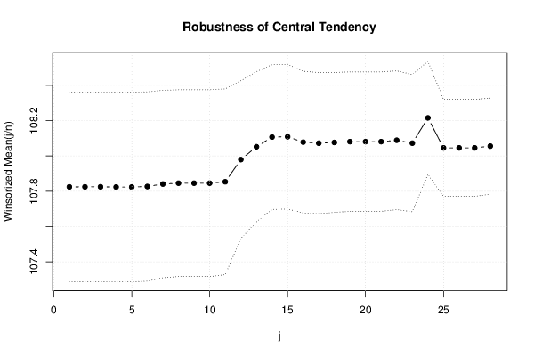
bitmap(file='test1.png')
lb <- win[,1] - 2*win[,2]
ub <- win[,1] + 2*win[,2]
if ((ylimmin == '') | (ylimmax == '')) plot(win[,1],type='b',main=main, xlab='j', pch=19, ylab='Winsorized Mean(j/n)', ylim=c(min(lb),max(ub))) else plot(win[,1],type='l',main=main, xlab='j', pch=19, ylab='Winsorized Mean(j/n)', ylim=c(ylimmin,ylimmax))
lines(ub,lty=3)
lines(lb,lty=3)
grid()
dev.off()
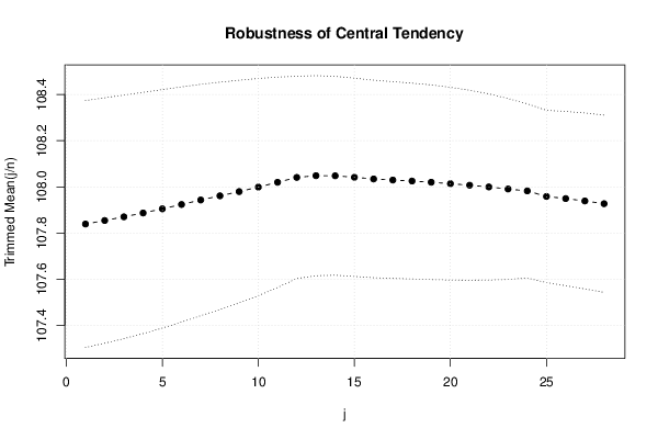
bitmap(file='test2.png')
lb <- tri[,1] - 2*tri[,2]
ub <- tri[,1] + 2*tri[,2]
if ((ylimmin == '') | (ylimmax == '')) plot(tri[,1],type='b',main=main, xlab='j', pch=19, ylab='Trimmed Mean(j/n)', ylim=c(min(lb),max(ub))) else plot(tri[,1],type='l',main=main, xlab='j', pch=19, ylab='Trimmed Mean(j/n)', ylim=c(ylimmin,ylimmax))
lines(ub,lty=3)
lines(lb,lty=3)
grid()
dev.off()
load(file='createtable')
a<-table.start()
a<-table.row.start(a)
a<-table.element(a,'Central Tendency - Ungrouped Data',4,TRUE)
a<-table.row.end(a)
a<-table.row.start(a)
a<-table.element(a,'Measure',header=TRUE)
a<-table.element(a,'Value',header=TRUE)
a<-table.element(a,'S.E.',header=TRUE)
a<-table.element(a,'Value/S.E.',header=TRUE)
a<-table.row.end(a)
a<-table.row.start(a)
a<-table.element(a,hyperlink('arithmetic_mean.htm', 'Arithmetic Mean', 'click to view the definition of the Arithmetic Mean'),header=TRUE)
a<-table.element(a,arm)
a<-table.element(a,hyperlink('arithmetic_mean_standard_error.htm', armse, 'click to view the definition of the Standard Error of the Arithmetic Mean'))
a<-table.element(a,armose)
a<-table.row.end(a)
a<-table.row.start(a)
a<-table.element(a,hyperlink('geometric_mean.htm', 'Geometric Mean', 'click to view the definition of the Geometric Mean'),header=TRUE)
a<-table.element(a,geo)
a<-table.element(a,'')
a<-table.row.end(a)
a<-table.row.start(a)
a<-table.element(a,hyperlink('harmonic_mean.htm', 'Harmonic Mean', 'click to view the definition of the Harmonic Mean'),header=TRUE)
a<-table.element(a,har)
a<-table.element(a,'')
a<-table.row.end(a)
a<-table.row.start(a)
a<-table.element(a,hyperlink('quadratic_mean.htm', 'Quadratic Mean', 'click to view the definition of the Quadratic Mean'),header=TRUE)
a<-table.element(a,qua)
a<-table.element(a,'')
a<-table.row.end(a)
for (j in 1:length(win[,1])) {
a<-table.row.start(a)
mylabel <- paste('Winsorized Mean (',j)
mylabel <- paste(mylabel,'/')
mylabel <- paste(mylabel,length(win[,1]))
mylabel <- paste(mylabel,')')
a<-table.element(a,hyperlink('winsorized_mean.htm', mylabel, 'click to view the definition of the Winsorized Mean'),header=TRUE)
a<-table.element(a,win[j,1])
a<-table.element(a,win[j,2])
a<-table.element(a,win[j,1]/win[j,2])
a<-table.row.end(a)
}
for (j in 1:length(tri[,1])) {
a<-table.row.start(a)
mylabel <- paste('Trimmed Mean (',j)
mylabel <- paste(mylabel,'/')
mylabel <- paste(mylabel,length(tri[,1]))
mylabel <- paste(mylabel,')')
a<-table.element(a,hyperlink('arithmetic_mean.htm', mylabel, 'click to view the definition of the Trimmed Mean'),header=TRUE)
a<-table.element(a,tri[j,1])
a<-table.element(a,tri[j,2])
a<-table.element(a,tri[j,1]/tri[j,2])
a<-table.row.end(a)
}
a<-table.row.start(a)
a<-table.element(a,hyperlink('median_1.htm', 'Median', 'click to view the definition of the Median'),header=TRUE)
a<-table.element(a,median(x))
a<-table.element(a,'')
a<-table.row.end(a)
a<-table.row.start(a)
a<-table.element(a,hyperlink('midrange.htm', 'Midrange', 'click to view the definition of the Midrange'),header=TRUE)
a<-table.element(a,midr)
a<-table.element(a,'')
a<-table.row.end(a)
a<-table.row.start(a)
mymid <- hyperlink('midmean.htm', 'Midmean', 'click to view the definition of the Midmean')
mylabel <- paste(mymid,hyperlink('method_1.htm','Weighted Average at Xnp',''),sep=' - ')
a<-table.element(a,mylabel,header=TRUE)
a<-table.element(a,midm[1])
a<-table.element(a,'')
a<-table.row.end(a)
a<-table.row.start(a)
mymid <- hyperlink('midmean.htm', 'Midmean', 'click to view the definition of the Midmean')
mylabel <- paste(mymid,hyperlink('method_2.htm','Weighted Average at X(n+1)p',''),sep=' - ')
a<-table.element(a,mylabel,header=TRUE)
a<-table.element(a,midm[2])
a<-table.element(a,'')
a<-table.row.end(a)
a<-table.row.start(a)
mymid <- hyperlink('midmean.htm', 'Midmean', 'click to view the definition of the Midmean')
mylabel <- paste(mymid,hyperlink('method_3.htm','Empirical Distribution Function',''),sep=' - ')
a<-table.element(a,mylabel,header=TRUE)
a<-table.element(a,midm[3])
a<-table.element(a,'')
a<-table.row.end(a)
a<-table.row.start(a)
mymid <- hyperlink('midmean.htm', 'Midmean', 'click to view the definition of the Midmean')
mylabel <- paste(mymid,hyperlink('method_4.htm','Empirical Distribution Function - Averaging',''),sep=' - ')
a<-table.element(a,mylabel,header=TRUE)
a<-table.element(a,midm[4])
a<-table.element(a,'')
a<-table.row.end(a)
a<-table.row.start(a)
mymid <- hyperlink('midmean.htm', 'Midmean', 'click to view the definition of the Midmean')
mylabel <- paste(mymid,hyperlink('method_5.htm','Empirical Distribution Function - Interpolation',''),sep=' - ')
a<-table.element(a,mylabel,header=TRUE)
a<-table.element(a,midm[5])
a<-table.element(a,'')
a<-table.row.end(a)
a<-table.row.start(a)
mymid <- hyperlink('midmean.htm', 'Midmean', 'click to view the definition of the Midmean')
mylabel <- paste(mymid,hyperlink('method_6.htm','Closest Observation',''),sep=' - ')
a<-table.element(a,mylabel,header=TRUE)
a<-table.element(a,midm[6])
a<-table.element(a,'')
a<-table.row.end(a)
a<-table.row.start(a)
mymid <- hyperlink('midmean.htm', 'Midmean', 'click to view the definition of the Midmean')
mylabel <- paste(mymid,hyperlink('method_7.htm','True Basic - Statistics Graphics Toolkit',''),sep=' - ')
a<-table.element(a,mylabel,header=TRUE)
a<-table.element(a,midm[7])
a<-table.element(a,'')
a<-table.row.end(a)
a<-table.row.start(a)
mymid <- hyperlink('midmean.htm', 'Midmean', 'click to view the definition of the Midmean')
mylabel <- paste(mymid,hyperlink('method_8.htm','MS Excel (old versions)',''),sep=' - ')
a<-table.element(a,mylabel,header=TRUE)
a<-table.element(a,midm[8])
a<-table.element(a,'')
a<-table.row.end(a)
a<-table.row.start(a)
a<-table.element(a,'Number of observations',header=TRUE)
a<-table.element(a,length(x))
a<-table.element(a,'')
a<-table.row.end(a)
a<-table.end(a)
table.save(a,file='mytable.tab')