Repository of Reproducible Computations

Free Statistics

of Irreproducible Research!

Author's title

Author

*Unverified author*

R Software Module

rwasp_autocorrelation.wasp

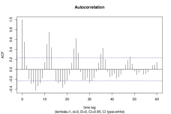
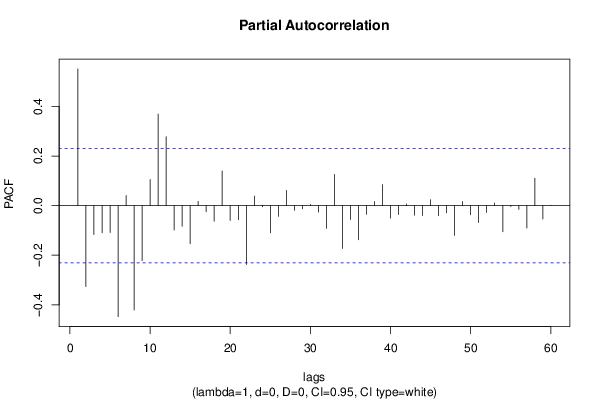
Title produced by software

(Partial) Autocorrelation Function

Date of computation

Fri, 10 Jan 2014 05:52:32 -0500

Cite this page as follows

Statistical Computations at FreeStatistics.org, Office for Research Development and Education, URL https://freestatistics.org/blog/index.php?v=date/2014/Jan/10/t1389351171qvisrbfyr7bihoj.htm/, Retrieved Sun, 19 May 2024 10:08:46 +0000

Statistical Computations at FreeStatistics.org, Office for Research Development and Education, URL https://freestatistics.org/blog/index.php?pk=232852, Retrieved Sun, 19 May 2024 10:08:46 +0000

QR Codes:

Paste this QR Code to cite your computation.

Original text written by user:

IsPrivate?

No (this computation is public)

User-defined keywords

Estimated Impact

157

Family? (F = Feedback message, R = changed R code, M = changed R Module, P = changed Parameters, D = changed Data)

-     [Notched Boxplots] [] [2014-01-10 09:41:38] [0b3be05215961a0fa3a77d7bd3c5f728]
- RMPD    [(Partial) Autocorrelation Function] [] [2014-01-10 10:52:32] [998078bdc1a977f0c7d195eebcf8b96b] [Current]
- R PD      [(Partial) Autocorrelation Function] [] [2014-01-10 11:01:02] [0b3be05215961a0fa3a77d7bd3c5f728] 
-    D      [(Partial) Autocorrelation Function] [] [2014-01-10 11:08:48] [0b3be05215961a0fa3a77d7bd3c5f728] 
- R PD        [(Partial) Autocorrelation Function] [] [2014-01-10 11:13:29] [0b3be05215961a0fa3a77d7bd3c5f728] 
- RMPD        [Classical Decomposition] [] [2014-01-10 12:34:21] [0b3be05215961a0fa3a77d7bd3c5f728] 
- RMPD      [Mean Plot] [] [2014-01-10 11:10:56] [0b3be05215961a0fa3a77d7bd3c5f728] 

Feedback Forum

Post a new message

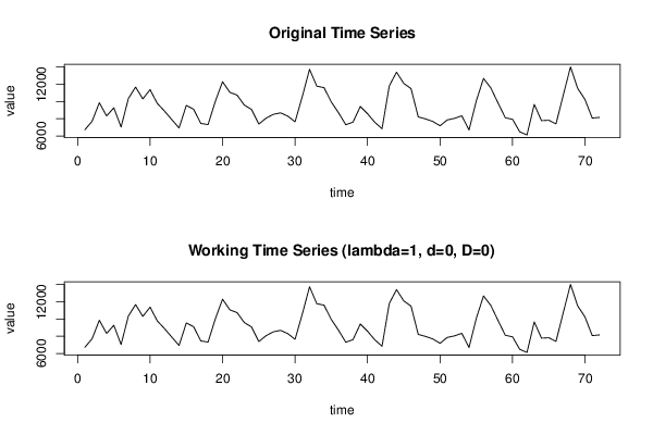
Dataseries X:

Download CSV

Histogram

Boxplots

6714,580043
7702,883281
9855,858483
8326,43136
9268,841212
7035,408602
10341,50586
11681,94192
10303,57287
11384,5829
9777,225921
8882,366455
7896,590139
6929,564098
9544,753788
9110,342185
7458,710291
7319,772861
10017,34419
12307,13647
11072,29609
10748,84755
9588,810984
9080,170402
7384,440407
8062,058679
8510,578229
8684,345395
8305,968153
7642,565124
10577,49554
13747,19397
11783,27459
11611,42999
9945,741914
8692,951724
7302,520182
7609,123374
9423,286031
8583,625656
7586,252878
6842,894335
11810,62427
13413,53598
12102,72578
11501,16989
8212,500701
7981,599542
7687
7180
7862
8043
8340
6692
10065
12684
11587
9843
8110
7940
6475
6121
9669
7778
7826
7403
10741
14023
11519
10236
8075
8157

Summary of computational transaction
Raw Input	view raw input (R code)
Raw Output	view raw output of R engine
Computing time	2 seconds
R Server	'George Udny Yule' @ yule.wessa.net

\begin{tabular}{lllllllll}
\hline
Summary of computational transaction \tabularnewline
Raw Input & view raw input (R code)  \tabularnewline
Raw Output & view raw output of R engine  \tabularnewline
Computing time & 2 seconds \tabularnewline
R Server & 'George Udny Yule' @ yule.wessa.net \tabularnewline
\hline
\end{tabular}
%Source: https://freestatistics.org/blog/index.php?pk=232852&T=0

[TABLE]
[ROW][C]Summary of computational transaction[/C][/ROW]
[ROW][C]Raw Input[/C][C]view raw input (R code) [/C][/ROW]
[ROW][C]Raw Output[/C][C]view raw output of R engine [/C][/ROW]
[ROW][C]Computing time[/C][C]2 seconds[/C][/ROW]
[ROW][C]R Server[/C][C]'George Udny Yule' @ yule.wessa.net[/C][/ROW]
[/TABLE]
Source: https://freestatistics.org/blog/index.php?pk=232852&T=0

Globally Unique Identifier (entire table): ba.freestatistics.org/blog/index.php?pk=232852&T=0

As an alternative you can also use a QR Code:

The GUIDs for individual cells are displayed in the table below:

Summary of computational transaction
Raw Input	view raw input (R code)
Raw Output	view raw output of R engine
Computing time	2 seconds
R Server	'George Udny Yule' @ yule.wessa.net

Autocorrelation Function
Time lag k	ACF(k)	T-STAT	P-value
1	0.551149	4.6767	7e-06
2	0.076694	0.6508	0.258632
3	-0.196252	-1.6653	0.050104
4	-0.286114	-2.4278	0.008847
5	-0.271707	-2.3055	0.012011
6	-0.421227	-3.5742	0.000316
7	-0.335869	-2.8499	0.00285
8	-0.274949	-2.333	0.011222
9	-0.175479	-1.489	0.070428
10	0.140504	1.1922	0.118546
11	0.508288	4.313	2.5e-05
12	0.747072	6.3391	0
13	0.439423	3.7286	0.00019
14	0.007786	0.0661	0.473753
15	-0.231217	-1.9619	0.026818
16	-0.27203	-2.3082	0.01193
17	-0.249402	-2.1162	0.018891
18	-0.364589	-3.0936	0.001407
19	-0.296334	-2.5145	0.007078
20	-0.222417	-1.8873	0.031577
21	-0.099284	-0.8425	0.201161
22	0.124551	1.0569	0.147057
23	0.412624	3.5012	4e-04
24	0.617889	5.243	1e-06
25	0.329527	2.7961	0.003314
26	-0.049119	-0.4168	0.339037
27	-0.218258	-1.852	0.034064
28	-0.212203	-1.8006	0.037977
29	-0.166678	-1.4143	0.08079
30	-0.266947	-2.2651	0.013258
31	-0.233454	-1.9809	0.02571
32	-0.172606	-1.4646	0.07369
33	-0.039761	-0.3374	0.368404
34	0.127818	1.0846	0.140864
35	0.30849	2.6176	0.005393
36	0.425485	3.6104	0.000281
37	0.199835	1.6957	0.047136
38	-0.042584	-0.3613	0.359453
39	-0.155122	-1.3163	0.096132
40	-0.124364	-1.0553	0.147416
41	-0.084224	-0.7147	0.238565
42	-0.180236	-1.5294	0.065279
43	-0.154295	-1.3092	0.097308
44	-0.098141	-0.8328	0.203868
45	-0.010349	-0.0878	0.465135
46	0.091467	0.7761	0.220108
47	0.181546	1.5405	0.063915
48	0.252209	2.1401	0.017869
49	0.106521	0.9039	0.184543
50	-0.035443	-0.3007	0.382239
51	-0.107851	-0.9151	0.181586
52	-0.060041	-0.5095	0.305993
53	-0.01396	-0.1185	0.453018
54	-0.100138	-0.8497	0.199155
55	-0.089104	-0.7561	0.226037
56	-0.057637	-0.4891	0.313142
57	-0.001076	-0.0091	0.496371
58	0.077649	0.6589	0.256039
59	0.087109	0.7391	0.231111
60	0.137218	1.1643	0.124067

\begin{tabular}{lllllllll}
\hline
Autocorrelation Function \tabularnewline
Time lag k & ACF(k) & T-STAT & P-value \tabularnewline
1 & 0.551149 & 4.6767 & 7e-06 \tabularnewline
2 & 0.076694 & 0.6508 & 0.258632 \tabularnewline
3 & -0.196252 & -1.6653 & 0.050104 \tabularnewline
4 & -0.286114 & -2.4278 & 0.008847 \tabularnewline
5 & -0.271707 & -2.3055 & 0.012011 \tabularnewline
6 & -0.421227 & -3.5742 & 0.000316 \tabularnewline
7 & -0.335869 & -2.8499 & 0.00285 \tabularnewline
8 & -0.274949 & -2.333 & 0.011222 \tabularnewline
9 & -0.175479 & -1.489 & 0.070428 \tabularnewline
10 & 0.140504 & 1.1922 & 0.118546 \tabularnewline
11 & 0.508288 & 4.313 & 2.5e-05 \tabularnewline
12 & 0.747072 & 6.3391 & 0 \tabularnewline
13 & 0.439423 & 3.7286 & 0.00019 \tabularnewline
14 & 0.007786 & 0.0661 & 0.473753 \tabularnewline
15 & -0.231217 & -1.9619 & 0.026818 \tabularnewline
16 & -0.27203 & -2.3082 & 0.01193 \tabularnewline
17 & -0.249402 & -2.1162 & 0.018891 \tabularnewline
18 & -0.364589 & -3.0936 & 0.001407 \tabularnewline
19 & -0.296334 & -2.5145 & 0.007078 \tabularnewline
20 & -0.222417 & -1.8873 & 0.031577 \tabularnewline
21 & -0.099284 & -0.8425 & 0.201161 \tabularnewline
22 & 0.124551 & 1.0569 & 0.147057 \tabularnewline
23 & 0.412624 & 3.5012 & 4e-04 \tabularnewline
24 & 0.617889 & 5.243 & 1e-06 \tabularnewline
25 & 0.329527 & 2.7961 & 0.003314 \tabularnewline
26 & -0.049119 & -0.4168 & 0.339037 \tabularnewline
27 & -0.218258 & -1.852 & 0.034064 \tabularnewline
28 & -0.212203 & -1.8006 & 0.037977 \tabularnewline
29 & -0.166678 & -1.4143 & 0.08079 \tabularnewline
30 & -0.266947 & -2.2651 & 0.013258 \tabularnewline
31 & -0.233454 & -1.9809 & 0.02571 \tabularnewline
32 & -0.172606 & -1.4646 & 0.07369 \tabularnewline
33 & -0.039761 & -0.3374 & 0.368404 \tabularnewline
34 & 0.127818 & 1.0846 & 0.140864 \tabularnewline
35 & 0.30849 & 2.6176 & 0.005393 \tabularnewline
36 & 0.425485 & 3.6104 & 0.000281 \tabularnewline
37 & 0.199835 & 1.6957 & 0.047136 \tabularnewline
38 & -0.042584 & -0.3613 & 0.359453 \tabularnewline
39 & -0.155122 & -1.3163 & 0.096132 \tabularnewline
40 & -0.124364 & -1.0553 & 0.147416 \tabularnewline
41 & -0.084224 & -0.7147 & 0.238565 \tabularnewline
42 & -0.180236 & -1.5294 & 0.065279 \tabularnewline
43 & -0.154295 & -1.3092 & 0.097308 \tabularnewline
44 & -0.098141 & -0.8328 & 0.203868 \tabularnewline
45 & -0.010349 & -0.0878 & 0.465135 \tabularnewline
46 & 0.091467 & 0.7761 & 0.220108 \tabularnewline
47 & 0.181546 & 1.5405 & 0.063915 \tabularnewline
48 & 0.252209 & 2.1401 & 0.017869 \tabularnewline
49 & 0.106521 & 0.9039 & 0.184543 \tabularnewline
50 & -0.035443 & -0.3007 & 0.382239 \tabularnewline
51 & -0.107851 & -0.9151 & 0.181586 \tabularnewline
52 & -0.060041 & -0.5095 & 0.305993 \tabularnewline
53 & -0.01396 & -0.1185 & 0.453018 \tabularnewline
54 & -0.100138 & -0.8497 & 0.199155 \tabularnewline
55 & -0.089104 & -0.7561 & 0.226037 \tabularnewline
56 & -0.057637 & -0.4891 & 0.313142 \tabularnewline
57 & -0.001076 & -0.0091 & 0.496371 \tabularnewline
58 & 0.077649 & 0.6589 & 0.256039 \tabularnewline
59 & 0.087109 & 0.7391 & 0.231111 \tabularnewline
60 & 0.137218 & 1.1643 & 0.124067 \tabularnewline
\hline
\end{tabular}
%Source: https://freestatistics.org/blog/index.php?pk=232852&T=1

[TABLE]
[ROW][C]Autocorrelation Function[/C][/ROW]
[ROW][C]Time lag k[/C][C]ACF(k)[/C][C]T-STAT[/C][C]P-value[/C][/ROW]
[ROW][C]1[/C][C]0.551149[/C][C]4.6767[/C][C]7e-06[/C][/ROW]
[ROW][C]2[/C][C]0.076694[/C][C]0.6508[/C][C]0.258632[/C][/ROW]
[ROW][C]3[/C][C]-0.196252[/C][C]-1.6653[/C][C]0.050104[/C][/ROW]
[ROW][C]4[/C][C]-0.286114[/C][C]-2.4278[/C][C]0.008847[/C][/ROW]
[ROW][C]5[/C][C]-0.271707[/C][C]-2.3055[/C][C]0.012011[/C][/ROW]
[ROW][C]6[/C][C]-0.421227[/C][C]-3.5742[/C][C]0.000316[/C][/ROW]
[ROW][C]7[/C][C]-0.335869[/C][C]-2.8499[/C][C]0.00285[/C][/ROW]
[ROW][C]8[/C][C]-0.274949[/C][C]-2.333[/C][C]0.011222[/C][/ROW]
[ROW][C]9[/C][C]-0.175479[/C][C]-1.489[/C][C]0.070428[/C][/ROW]
[ROW][C]10[/C][C]0.140504[/C][C]1.1922[/C][C]0.118546[/C][/ROW]
[ROW][C]11[/C][C]0.508288[/C][C]4.313[/C][C]2.5e-05[/C][/ROW]
[ROW][C]12[/C][C]0.747072[/C][C]6.3391[/C][C]0[/C][/ROW]
[ROW][C]13[/C][C]0.439423[/C][C]3.7286[/C][C]0.00019[/C][/ROW]
[ROW][C]14[/C][C]0.007786[/C][C]0.0661[/C][C]0.473753[/C][/ROW]
[ROW][C]15[/C][C]-0.231217[/C][C]-1.9619[/C][C]0.026818[/C][/ROW]
[ROW][C]16[/C][C]-0.27203[/C][C]-2.3082[/C][C]0.01193[/C][/ROW]
[ROW][C]17[/C][C]-0.249402[/C][C]-2.1162[/C][C]0.018891[/C][/ROW]
[ROW][C]18[/C][C]-0.364589[/C][C]-3.0936[/C][C]0.001407[/C][/ROW]
[ROW][C]19[/C][C]-0.296334[/C][C]-2.5145[/C][C]0.007078[/C][/ROW]
[ROW][C]20[/C][C]-0.222417[/C][C]-1.8873[/C][C]0.031577[/C][/ROW]
[ROW][C]21[/C][C]-0.099284[/C][C]-0.8425[/C][C]0.201161[/C][/ROW]
[ROW][C]22[/C][C]0.124551[/C][C]1.0569[/C][C]0.147057[/C][/ROW]
[ROW][C]23[/C][C]0.412624[/C][C]3.5012[/C][C]4e-04[/C][/ROW]
[ROW][C]24[/C][C]0.617889[/C][C]5.243[/C][C]1e-06[/C][/ROW]
[ROW][C]25[/C][C]0.329527[/C][C]2.7961[/C][C]0.003314[/C][/ROW]
[ROW][C]26[/C][C]-0.049119[/C][C]-0.4168[/C][C]0.339037[/C][/ROW]
[ROW][C]27[/C][C]-0.218258[/C][C]-1.852[/C][C]0.034064[/C][/ROW]
[ROW][C]28[/C][C]-0.212203[/C][C]-1.8006[/C][C]0.037977[/C][/ROW]
[ROW][C]29[/C][C]-0.166678[/C][C]-1.4143[/C][C]0.08079[/C][/ROW]
[ROW][C]30[/C][C]-0.266947[/C][C]-2.2651[/C][C]0.013258[/C][/ROW]
[ROW][C]31[/C][C]-0.233454[/C][C]-1.9809[/C][C]0.02571[/C][/ROW]
[ROW][C]32[/C][C]-0.172606[/C][C]-1.4646[/C][C]0.07369[/C][/ROW]
[ROW][C]33[/C][C]-0.039761[/C][C]-0.3374[/C][C]0.368404[/C][/ROW]
[ROW][C]34[/C][C]0.127818[/C][C]1.0846[/C][C]0.140864[/C][/ROW]
[ROW][C]35[/C][C]0.30849[/C][C]2.6176[/C][C]0.005393[/C][/ROW]
[ROW][C]36[/C][C]0.425485[/C][C]3.6104[/C][C]0.000281[/C][/ROW]
[ROW][C]37[/C][C]0.199835[/C][C]1.6957[/C][C]0.047136[/C][/ROW]
[ROW][C]38[/C][C]-0.042584[/C][C]-0.3613[/C][C]0.359453[/C][/ROW]
[ROW][C]39[/C][C]-0.155122[/C][C]-1.3163[/C][C]0.096132[/C][/ROW]
[ROW][C]40[/C][C]-0.124364[/C][C]-1.0553[/C][C]0.147416[/C][/ROW]
[ROW][C]41[/C][C]-0.084224[/C][C]-0.7147[/C][C]0.238565[/C][/ROW]
[ROW][C]42[/C][C]-0.180236[/C][C]-1.5294[/C][C]0.065279[/C][/ROW]
[ROW][C]43[/C][C]-0.154295[/C][C]-1.3092[/C][C]0.097308[/C][/ROW]
[ROW][C]44[/C][C]-0.098141[/C][C]-0.8328[/C][C]0.203868[/C][/ROW]
[ROW][C]45[/C][C]-0.010349[/C][C]-0.0878[/C][C]0.465135[/C][/ROW]
[ROW][C]46[/C][C]0.091467[/C][C]0.7761[/C][C]0.220108[/C][/ROW]
[ROW][C]47[/C][C]0.181546[/C][C]1.5405[/C][C]0.063915[/C][/ROW]
[ROW][C]48[/C][C]0.252209[/C][C]2.1401[/C][C]0.017869[/C][/ROW]
[ROW][C]49[/C][C]0.106521[/C][C]0.9039[/C][C]0.184543[/C][/ROW]
[ROW][C]50[/C][C]-0.035443[/C][C]-0.3007[/C][C]0.382239[/C][/ROW]
[ROW][C]51[/C][C]-0.107851[/C][C]-0.9151[/C][C]0.181586[/C][/ROW]
[ROW][C]52[/C][C]-0.060041[/C][C]-0.5095[/C][C]0.305993[/C][/ROW]
[ROW][C]53[/C][C]-0.01396[/C][C]-0.1185[/C][C]0.453018[/C][/ROW]
[ROW][C]54[/C][C]-0.100138[/C][C]-0.8497[/C][C]0.199155[/C][/ROW]
[ROW][C]55[/C][C]-0.089104[/C][C]-0.7561[/C][C]0.226037[/C][/ROW]
[ROW][C]56[/C][C]-0.057637[/C][C]-0.4891[/C][C]0.313142[/C][/ROW]
[ROW][C]57[/C][C]-0.001076[/C][C]-0.0091[/C][C]0.496371[/C][/ROW]
[ROW][C]58[/C][C]0.077649[/C][C]0.6589[/C][C]0.256039[/C][/ROW]
[ROW][C]59[/C][C]0.087109[/C][C]0.7391[/C][C]0.231111[/C][/ROW]
[ROW][C]60[/C][C]0.137218[/C][C]1.1643[/C][C]0.124067[/C][/ROW]
[/TABLE]
Source: https://freestatistics.org/blog/index.php?pk=232852&T=1

Globally Unique Identifier (entire table): ba.freestatistics.org/blog/index.php?pk=232852&T=1

As an alternative you can also use a QR Code:

The GUIDs for individual cells are displayed in the table below:

Autocorrelation Function
Time lag k	ACF(k)	T-STAT	P-value
1	0.551149	4.6767	7e-06
2	0.076694	0.6508	0.258632
3	-0.196252	-1.6653	0.050104
4	-0.286114	-2.4278	0.008847
5	-0.271707	-2.3055	0.012011
6	-0.421227	-3.5742	0.000316
7	-0.335869	-2.8499	0.00285
8	-0.274949	-2.333	0.011222
9	-0.175479	-1.489	0.070428
10	0.140504	1.1922	0.118546
11	0.508288	4.313	2.5e-05
12	0.747072	6.3391	0
13	0.439423	3.7286	0.00019
14	0.007786	0.0661	0.473753
15	-0.231217	-1.9619	0.026818
16	-0.27203	-2.3082	0.01193
17	-0.249402	-2.1162	0.018891
18	-0.364589	-3.0936	0.001407
19	-0.296334	-2.5145	0.007078
20	-0.222417	-1.8873	0.031577
21	-0.099284	-0.8425	0.201161
22	0.124551	1.0569	0.147057
23	0.412624	3.5012	4e-04
24	0.617889	5.243	1e-06
25	0.329527	2.7961	0.003314
26	-0.049119	-0.4168	0.339037
27	-0.218258	-1.852	0.034064
28	-0.212203	-1.8006	0.037977
29	-0.166678	-1.4143	0.08079
30	-0.266947	-2.2651	0.013258
31	-0.233454	-1.9809	0.02571
32	-0.172606	-1.4646	0.07369
33	-0.039761	-0.3374	0.368404
34	0.127818	1.0846	0.140864
35	0.30849	2.6176	0.005393
36	0.425485	3.6104	0.000281
37	0.199835	1.6957	0.047136
38	-0.042584	-0.3613	0.359453
39	-0.155122	-1.3163	0.096132
40	-0.124364	-1.0553	0.147416
41	-0.084224	-0.7147	0.238565
42	-0.180236	-1.5294	0.065279
43	-0.154295	-1.3092	0.097308
44	-0.098141	-0.8328	0.203868
45	-0.010349	-0.0878	0.465135
46	0.091467	0.7761	0.220108
47	0.181546	1.5405	0.063915
48	0.252209	2.1401	0.017869
49	0.106521	0.9039	0.184543
50	-0.035443	-0.3007	0.382239
51	-0.107851	-0.9151	0.181586
52	-0.060041	-0.5095	0.305993
53	-0.01396	-0.1185	0.453018
54	-0.100138	-0.8497	0.199155
55	-0.089104	-0.7561	0.226037
56	-0.057637	-0.4891	0.313142
57	-0.001076	-0.0091	0.496371
58	0.077649	0.6589	0.256039
59	0.087109	0.7391	0.231111
60	0.137218	1.1643	0.124067

Partial Autocorrelation Function
Time lag k	PACF(k)	T-STAT	P-value
1	0.551149	4.6767	7e-06
2	-0.326141	-2.7674	0.003589
3	-0.116616	-0.9895	0.162862
4	-0.109804	-0.9317	0.177298
5	-0.108811	-0.9233	0.179469
6	-0.447976	-3.8012	0.000149
7	0.040411	0.3429	0.366335
8	-0.420861	-3.5711	0.000319
9	-0.222015	-1.8839	0.031811
10	0.105401	0.8944	0.187056
11	0.368907	3.1303	0.001261
12	0.277696	2.3563	0.01059
13	-0.098461	-0.8355	0.20311
14	-0.083339	-0.7072	0.240876
15	-0.154227	-1.3087	0.097406
16	0.016899	0.1434	0.443191
17	-0.024855	-0.2109	0.41678
18	-0.062771	-0.5326	0.297964
19	0.139485	1.1836	0.120239
20	-0.059896	-0.5082	0.306422
21	-0.056763	-0.4817	0.315758
22	-0.237406	-2.0145	0.023849
23	0.038097	0.3233	0.373718
24	-0.004539	-0.0385	0.484692
25	-0.109462	-0.9288	0.178045
26	-0.0434	-0.3683	0.356881
27	0.061099	0.5184	0.30287
28	-0.018883	-0.1602	0.436575
29	-0.012765	-0.1083	0.457025
30	0.004166	0.0354	0.485948
31	-0.02627	-0.2229	0.412118
32	-0.091852	-0.7794	0.219151
33	0.125165	1.0621	0.145879
34	-0.173248	-1.4701	0.072951
35	-0.056176	-0.4767	0.317522
36	-0.137623	-1.1678	0.123376
37	-0.035307	-0.2996	0.382678
38	0.016754	0.1422	0.443675
39	0.084534	0.7173	0.237757
40	-0.050632	-0.4296	0.334375
41	-0.036064	-0.306	0.380238
42	0.006521	0.0553	0.478013
43	-0.038606	-0.3276	0.37209
44	-0.040072	-0.34	0.367415
45	0.023258	0.1974	0.422055
46	-0.040421	-0.343	0.366304
47	-0.02907	-0.2467	0.402935
48	-0.120253	-1.0204	0.155482
49	0.016851	0.143	0.44335
50	-0.037072	-0.3146	0.377001
51	-0.068321	-0.5797	0.281956
52	-0.027644	-0.2346	0.407605
53	0.010343	0.0878	0.465153
54	-0.105832	-0.898	0.186086
55	-0.003617	-0.0307	0.487801
56	-0.01547	-0.1313	0.447964
57	-0.090491	-0.7678	0.222547
58	0.110298	0.9359	0.176225
59	-0.054085	-0.4589	0.323834
60	0.001226	0.0104	0.495863

\begin{tabular}{lllllllll}
\hline
Partial Autocorrelation Function \tabularnewline
Time lag k & PACF(k) & T-STAT & P-value \tabularnewline
1 & 0.551149 & 4.6767 & 7e-06 \tabularnewline
2 & -0.326141 & -2.7674 & 0.003589 \tabularnewline
3 & -0.116616 & -0.9895 & 0.162862 \tabularnewline
4 & -0.109804 & -0.9317 & 0.177298 \tabularnewline
5 & -0.108811 & -0.9233 & 0.179469 \tabularnewline
6 & -0.447976 & -3.8012 & 0.000149 \tabularnewline
7 & 0.040411 & 0.3429 & 0.366335 \tabularnewline
8 & -0.420861 & -3.5711 & 0.000319 \tabularnewline
9 & -0.222015 & -1.8839 & 0.031811 \tabularnewline
10 & 0.105401 & 0.8944 & 0.187056 \tabularnewline
11 & 0.368907 & 3.1303 & 0.001261 \tabularnewline
12 & 0.277696 & 2.3563 & 0.01059 \tabularnewline
13 & -0.098461 & -0.8355 & 0.20311 \tabularnewline
14 & -0.083339 & -0.7072 & 0.240876 \tabularnewline
15 & -0.154227 & -1.3087 & 0.097406 \tabularnewline
16 & 0.016899 & 0.1434 & 0.443191 \tabularnewline
17 & -0.024855 & -0.2109 & 0.41678 \tabularnewline
18 & -0.062771 & -0.5326 & 0.297964 \tabularnewline
19 & 0.139485 & 1.1836 & 0.120239 \tabularnewline
20 & -0.059896 & -0.5082 & 0.306422 \tabularnewline
21 & -0.056763 & -0.4817 & 0.315758 \tabularnewline
22 & -0.237406 & -2.0145 & 0.023849 \tabularnewline
23 & 0.038097 & 0.3233 & 0.373718 \tabularnewline
24 & -0.004539 & -0.0385 & 0.484692 \tabularnewline
25 & -0.109462 & -0.9288 & 0.178045 \tabularnewline
26 & -0.0434 & -0.3683 & 0.356881 \tabularnewline
27 & 0.061099 & 0.5184 & 0.30287 \tabularnewline
28 & -0.018883 & -0.1602 & 0.436575 \tabularnewline
29 & -0.012765 & -0.1083 & 0.457025 \tabularnewline
30 & 0.004166 & 0.0354 & 0.485948 \tabularnewline
31 & -0.02627 & -0.2229 & 0.412118 \tabularnewline
32 & -0.091852 & -0.7794 & 0.219151 \tabularnewline
33 & 0.125165 & 1.0621 & 0.145879 \tabularnewline
34 & -0.173248 & -1.4701 & 0.072951 \tabularnewline
35 & -0.056176 & -0.4767 & 0.317522 \tabularnewline
36 & -0.137623 & -1.1678 & 0.123376 \tabularnewline
37 & -0.035307 & -0.2996 & 0.382678 \tabularnewline
38 & 0.016754 & 0.1422 & 0.443675 \tabularnewline
39 & 0.084534 & 0.7173 & 0.237757 \tabularnewline
40 & -0.050632 & -0.4296 & 0.334375 \tabularnewline
41 & -0.036064 & -0.306 & 0.380238 \tabularnewline
42 & 0.006521 & 0.0553 & 0.478013 \tabularnewline
43 & -0.038606 & -0.3276 & 0.37209 \tabularnewline
44 & -0.040072 & -0.34 & 0.367415 \tabularnewline
45 & 0.023258 & 0.1974 & 0.422055 \tabularnewline
46 & -0.040421 & -0.343 & 0.366304 \tabularnewline
47 & -0.02907 & -0.2467 & 0.402935 \tabularnewline
48 & -0.120253 & -1.0204 & 0.155482 \tabularnewline
49 & 0.016851 & 0.143 & 0.44335 \tabularnewline
50 & -0.037072 & -0.3146 & 0.377001 \tabularnewline
51 & -0.068321 & -0.5797 & 0.281956 \tabularnewline
52 & -0.027644 & -0.2346 & 0.407605 \tabularnewline
53 & 0.010343 & 0.0878 & 0.465153 \tabularnewline
54 & -0.105832 & -0.898 & 0.186086 \tabularnewline
55 & -0.003617 & -0.0307 & 0.487801 \tabularnewline
56 & -0.01547 & -0.1313 & 0.447964 \tabularnewline
57 & -0.090491 & -0.7678 & 0.222547 \tabularnewline
58 & 0.110298 & 0.9359 & 0.176225 \tabularnewline
59 & -0.054085 & -0.4589 & 0.323834 \tabularnewline
60 & 0.001226 & 0.0104 & 0.495863 \tabularnewline
\hline
\end{tabular}
%Source: https://freestatistics.org/blog/index.php?pk=232852&T=2

[TABLE]
[ROW][C]Partial Autocorrelation Function[/C][/ROW]
[ROW][C]Time lag k[/C][C]PACF(k)[/C][C]T-STAT[/C][C]P-value[/C][/ROW]
[ROW][C]1[/C][C]0.551149[/C][C]4.6767[/C][C]7e-06[/C][/ROW]
[ROW][C]2[/C][C]-0.326141[/C][C]-2.7674[/C][C]0.003589[/C][/ROW]
[ROW][C]3[/C][C]-0.116616[/C][C]-0.9895[/C][C]0.162862[/C][/ROW]
[ROW][C]4[/C][C]-0.109804[/C][C]-0.9317[/C][C]0.177298[/C][/ROW]
[ROW][C]5[/C][C]-0.108811[/C][C]-0.9233[/C][C]0.179469[/C][/ROW]
[ROW][C]6[/C][C]-0.447976[/C][C]-3.8012[/C][C]0.000149[/C][/ROW]
[ROW][C]7[/C][C]0.040411[/C][C]0.3429[/C][C]0.366335[/C][/ROW]
[ROW][C]8[/C][C]-0.420861[/C][C]-3.5711[/C][C]0.000319[/C][/ROW]
[ROW][C]9[/C][C]-0.222015[/C][C]-1.8839[/C][C]0.031811[/C][/ROW]
[ROW][C]10[/C][C]0.105401[/C][C]0.8944[/C][C]0.187056[/C][/ROW]
[ROW][C]11[/C][C]0.368907[/C][C]3.1303[/C][C]0.001261[/C][/ROW]
[ROW][C]12[/C][C]0.277696[/C][C]2.3563[/C][C]0.01059[/C][/ROW]
[ROW][C]13[/C][C]-0.098461[/C][C]-0.8355[/C][C]0.20311[/C][/ROW]
[ROW][C]14[/C][C]-0.083339[/C][C]-0.7072[/C][C]0.240876[/C][/ROW]
[ROW][C]15[/C][C]-0.154227[/C][C]-1.3087[/C][C]0.097406[/C][/ROW]
[ROW][C]16[/C][C]0.016899[/C][C]0.1434[/C][C]0.443191[/C][/ROW]
[ROW][C]17[/C][C]-0.024855[/C][C]-0.2109[/C][C]0.41678[/C][/ROW]
[ROW][C]18[/C][C]-0.062771[/C][C]-0.5326[/C][C]0.297964[/C][/ROW]
[ROW][C]19[/C][C]0.139485[/C][C]1.1836[/C][C]0.120239[/C][/ROW]
[ROW][C]20[/C][C]-0.059896[/C][C]-0.5082[/C][C]0.306422[/C][/ROW]
[ROW][C]21[/C][C]-0.056763[/C][C]-0.4817[/C][C]0.315758[/C][/ROW]
[ROW][C]22[/C][C]-0.237406[/C][C]-2.0145[/C][C]0.023849[/C][/ROW]
[ROW][C]23[/C][C]0.038097[/C][C]0.3233[/C][C]0.373718[/C][/ROW]
[ROW][C]24[/C][C]-0.004539[/C][C]-0.0385[/C][C]0.484692[/C][/ROW]
[ROW][C]25[/C][C]-0.109462[/C][C]-0.9288[/C][C]0.178045[/C][/ROW]
[ROW][C]26[/C][C]-0.0434[/C][C]-0.3683[/C][C]0.356881[/C][/ROW]
[ROW][C]27[/C][C]0.061099[/C][C]0.5184[/C][C]0.30287[/C][/ROW]
[ROW][C]28[/C][C]-0.018883[/C][C]-0.1602[/C][C]0.436575[/C][/ROW]
[ROW][C]29[/C][C]-0.012765[/C][C]-0.1083[/C][C]0.457025[/C][/ROW]
[ROW][C]30[/C][C]0.004166[/C][C]0.0354[/C][C]0.485948[/C][/ROW]
[ROW][C]31[/C][C]-0.02627[/C][C]-0.2229[/C][C]0.412118[/C][/ROW]
[ROW][C]32[/C][C]-0.091852[/C][C]-0.7794[/C][C]0.219151[/C][/ROW]
[ROW][C]33[/C][C]0.125165[/C][C]1.0621[/C][C]0.145879[/C][/ROW]
[ROW][C]34[/C][C]-0.173248[/C][C]-1.4701[/C][C]0.072951[/C][/ROW]
[ROW][C]35[/C][C]-0.056176[/C][C]-0.4767[/C][C]0.317522[/C][/ROW]
[ROW][C]36[/C][C]-0.137623[/C][C]-1.1678[/C][C]0.123376[/C][/ROW]
[ROW][C]37[/C][C]-0.035307[/C][C]-0.2996[/C][C]0.382678[/C][/ROW]
[ROW][C]38[/C][C]0.016754[/C][C]0.1422[/C][C]0.443675[/C][/ROW]
[ROW][C]39[/C][C]0.084534[/C][C]0.7173[/C][C]0.237757[/C][/ROW]
[ROW][C]40[/C][C]-0.050632[/C][C]-0.4296[/C][C]0.334375[/C][/ROW]
[ROW][C]41[/C][C]-0.036064[/C][C]-0.306[/C][C]0.380238[/C][/ROW]
[ROW][C]42[/C][C]0.006521[/C][C]0.0553[/C][C]0.478013[/C][/ROW]
[ROW][C]43[/C][C]-0.038606[/C][C]-0.3276[/C][C]0.37209[/C][/ROW]
[ROW][C]44[/C][C]-0.040072[/C][C]-0.34[/C][C]0.367415[/C][/ROW]
[ROW][C]45[/C][C]0.023258[/C][C]0.1974[/C][C]0.422055[/C][/ROW]
[ROW][C]46[/C][C]-0.040421[/C][C]-0.343[/C][C]0.366304[/C][/ROW]
[ROW][C]47[/C][C]-0.02907[/C][C]-0.2467[/C][C]0.402935[/C][/ROW]
[ROW][C]48[/C][C]-0.120253[/C][C]-1.0204[/C][C]0.155482[/C][/ROW]
[ROW][C]49[/C][C]0.016851[/C][C]0.143[/C][C]0.44335[/C][/ROW]
[ROW][C]50[/C][C]-0.037072[/C][C]-0.3146[/C][C]0.377001[/C][/ROW]
[ROW][C]51[/C][C]-0.068321[/C][C]-0.5797[/C][C]0.281956[/C][/ROW]
[ROW][C]52[/C][C]-0.027644[/C][C]-0.2346[/C][C]0.407605[/C][/ROW]
[ROW][C]53[/C][C]0.010343[/C][C]0.0878[/C][C]0.465153[/C][/ROW]
[ROW][C]54[/C][C]-0.105832[/C][C]-0.898[/C][C]0.186086[/C][/ROW]
[ROW][C]55[/C][C]-0.003617[/C][C]-0.0307[/C][C]0.487801[/C][/ROW]
[ROW][C]56[/C][C]-0.01547[/C][C]-0.1313[/C][C]0.447964[/C][/ROW]
[ROW][C]57[/C][C]-0.090491[/C][C]-0.7678[/C][C]0.222547[/C][/ROW]
[ROW][C]58[/C][C]0.110298[/C][C]0.9359[/C][C]0.176225[/C][/ROW]
[ROW][C]59[/C][C]-0.054085[/C][C]-0.4589[/C][C]0.323834[/C][/ROW]
[ROW][C]60[/C][C]0.001226[/C][C]0.0104[/C][C]0.495863[/C][/ROW]
[/TABLE]
Source: https://freestatistics.org/blog/index.php?pk=232852&T=2

Globally Unique Identifier (entire table): ba.freestatistics.org/blog/index.php?pk=232852&T=2

As an alternative you can also use a QR Code:

The GUIDs for individual cells are displayed in the table below:

Partial Autocorrelation Function
Time lag k	PACF(k)	T-STAT	P-value
1	0.551149	4.6767	7e-06
2	-0.326141	-2.7674	0.003589
3	-0.116616	-0.9895	0.162862
4	-0.109804	-0.9317	0.177298
5	-0.108811	-0.9233	0.179469
6	-0.447976	-3.8012	0.000149
7	0.040411	0.3429	0.366335
8	-0.420861	-3.5711	0.000319
9	-0.222015	-1.8839	0.031811
10	0.105401	0.8944	0.187056
11	0.368907	3.1303	0.001261
12	0.277696	2.3563	0.01059
13	-0.098461	-0.8355	0.20311
14	-0.083339	-0.7072	0.240876
15	-0.154227	-1.3087	0.097406
16	0.016899	0.1434	0.443191
17	-0.024855	-0.2109	0.41678
18	-0.062771	-0.5326	0.297964
19	0.139485	1.1836	0.120239
20	-0.059896	-0.5082	0.306422
21	-0.056763	-0.4817	0.315758
22	-0.237406	-2.0145	0.023849
23	0.038097	0.3233	0.373718
24	-0.004539	-0.0385	0.484692
25	-0.109462	-0.9288	0.178045
26	-0.0434	-0.3683	0.356881
27	0.061099	0.5184	0.30287
28	-0.018883	-0.1602	0.436575
29	-0.012765	-0.1083	0.457025
30	0.004166	0.0354	0.485948
31	-0.02627	-0.2229	0.412118
32	-0.091852	-0.7794	0.219151
33	0.125165	1.0621	0.145879
34	-0.173248	-1.4701	0.072951
35	-0.056176	-0.4767	0.317522
36	-0.137623	-1.1678	0.123376
37	-0.035307	-0.2996	0.382678
38	0.016754	0.1422	0.443675
39	0.084534	0.7173	0.237757
40	-0.050632	-0.4296	0.334375
41	-0.036064	-0.306	0.380238
42	0.006521	0.0553	0.478013
43	-0.038606	-0.3276	0.37209
44	-0.040072	-0.34	0.367415
45	0.023258	0.1974	0.422055
46	-0.040421	-0.343	0.366304
47	-0.02907	-0.2467	0.402935
48	-0.120253	-1.0204	0.155482
49	0.016851	0.143	0.44335
50	-0.037072	-0.3146	0.377001
51	-0.068321	-0.5797	0.281956
52	-0.027644	-0.2346	0.407605
53	0.010343	0.0878	0.465153
54	-0.105832	-0.898	0.186086
55	-0.003617	-0.0307	0.487801
56	-0.01547	-0.1313	0.447964
57	-0.090491	-0.7678	0.222547
58	0.110298	0.9359	0.176225
59	-0.054085	-0.4589	0.323834
60	0.001226	0.0104	0.495863

Figure 1

PNG link

Postscript link

PDF link

Figure 2

PNG link

Postscript link

PDF link

Figure 3

PNG link

Postscript link

PDF link

Parameters (Session):

par1 = 60 ; par2 = 1 ; par3 = 0 ; par4 = 0 ; par5 = 12 ; par6 = White Noise ; par7 = 0.95 ;

Parameters (R input):

par1 = 60 ; par2 = 1 ; par3 = 0 ; par4 = 0 ; par5 = 12 ; par6 = White Noise ; par7 = 0.95 ; par8 = ;

R code (references can be found in the software module):

if (par1 == 'Default') {
par1 = 10*log10(length(x))
} else {
par1 <- as.numeric(par1)
}
par2 <- as.numeric(par2)
par3 <- as.numeric(par3)
par4 <- as.numeric(par4)
par5 <- as.numeric(par5)
if (par6 == 'White Noise') par6 <- 'white' else par6 <- 'ma'
par7 <- as.numeric(par7)
if (par8 != '') par8 <- as.numeric(par8)
ox <- x
if (par8 == '') {
if (par2 == 0) {
x <- log(x)
} else {
x <- (x ^ par2 - 1) / par2
}
} else {
x <- log(x,base=par8)
}
if (par3 > 0) x <- diff(x,lag=1,difference=par3)
if (par4 > 0) x <- diff(x,lag=par5,difference=par4)
bitmap(file='picts.png')
op <- par(mfrow=c(2,1))
plot(ox,type='l',main='Original Time Series',xlab='time',ylab='value')
if (par8=='') {
mytitle <- paste('Working Time Series (lambda=',par2,', d=',par3,', D=',par4,')',sep='')
mysub <- paste('(lambda=',par2,', d=',par3,', D=',par4,', CI=', par7, ', CI type=',par6,')',sep='')
} else {
mytitle <- paste('Working Time Series (base=',par8,', d=',par3,', D=',par4,')',sep='')
mysub <- paste('(base=',par8,', d=',par3,', D=',par4,', CI=', par7, ', CI type=',par6,')',sep='')
}
plot(x,type='l', main=mytitle,xlab='time',ylab='value')
par(op)
dev.off()
bitmap(file='pic1.png')
racf <- acf(x, par1, main='Autocorrelation', xlab='time lag', ylab='ACF', ci.type=par6, ci=par7, sub=mysub)
dev.off()
bitmap(file='pic2.png')
rpacf <- pacf(x,par1,main='Partial Autocorrelation',xlab='lags',ylab='PACF',sub=mysub)
dev.off()
(myacf <- c(racf$acf))
(mypacf <- c(rpacf$acf))
lengthx <- length(x)
sqrtn <- sqrt(lengthx)
load(file='createtable')
a<-table.start()
a<-table.row.start(a)
a<-table.element(a,'Autocorrelation Function',4,TRUE)
a<-table.row.end(a)
a<-table.row.start(a)
a<-table.element(a,'Time lag k',header=TRUE)
a<-table.element(a,hyperlink('basics.htm','ACF(k)','click here for more information about the Autocorrelation Function'),header=TRUE)
a<-table.element(a,'T-STAT',header=TRUE)
a<-table.element(a,'P-value',header=TRUE)
a<-table.row.end(a)
for (i in 2:(par1+1)) {
a<-table.row.start(a)
a<-table.element(a,i-1,header=TRUE)
a<-table.element(a,round(myacf[i],6))
mytstat <- myacf[i]*sqrtn
a<-table.element(a,round(mytstat,4))
a<-table.element(a,round(1-pt(abs(mytstat),lengthx),6))
a<-table.row.end(a)
}
a<-table.end(a)
table.save(a,file='mytable.tab')
a<-table.start()
a<-table.row.start(a)
a<-table.element(a,'Partial Autocorrelation Function',4,TRUE)
a<-table.row.end(a)
a<-table.row.start(a)
a<-table.element(a,'Time lag k',header=TRUE)
a<-table.element(a,hyperlink('basics.htm','PACF(k)','click here for more information about the Partial Autocorrelation Function'),header=TRUE)
a<-table.element(a,'T-STAT',header=TRUE)
a<-table.element(a,'P-value',header=TRUE)
a<-table.row.end(a)
for (i in 1:par1) {
a<-table.row.start(a)
a<-table.element(a,i,header=TRUE)
a<-table.element(a,round(mypacf[i],6))
mytstat <- mypacf[i]*sqrtn
a<-table.element(a,round(mytstat,4))
a<-table.element(a,round(1-pt(abs(mytstat),lengthx),6))
a<-table.row.end(a)
}
a<-table.end(a)
table.save(a,file='mytable1.tab')

Free Statistics

Description of Statistical Computation

Tree of Dependent Computations

Dataset

Tables (Output of Computation)

Figures (Output of Computation)

Input Parameters & R Code