Repository of Reproducible Computations

Free Statistics

of Irreproducible Research!

Author's title

Author

*The author of this computation has been verified*

R Software Module

rwasp_bootstrapplot1.wasp

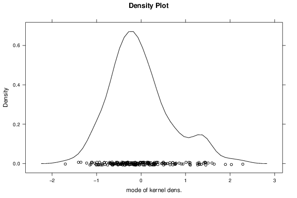
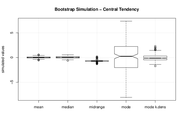
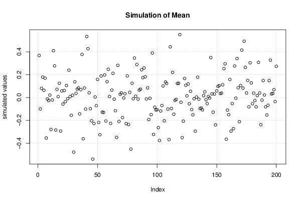
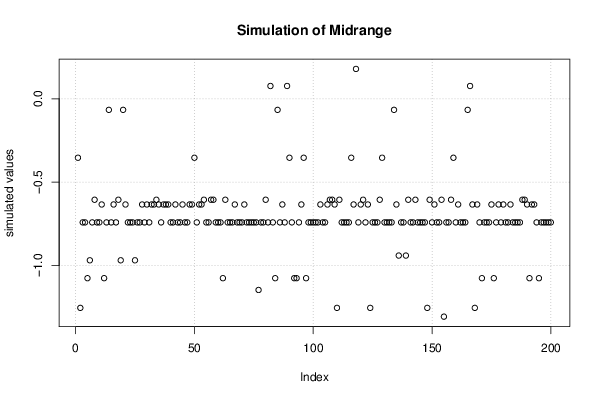
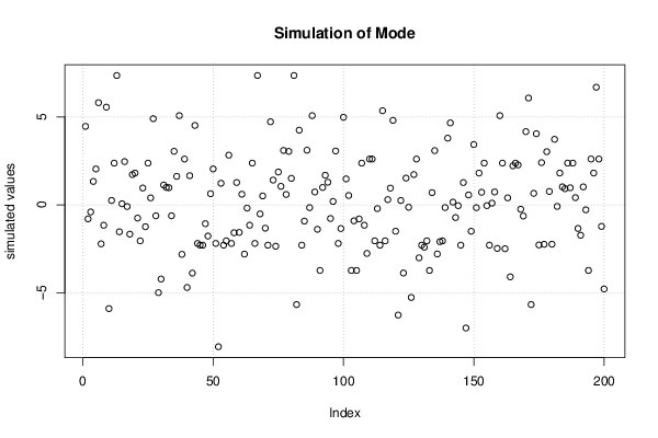
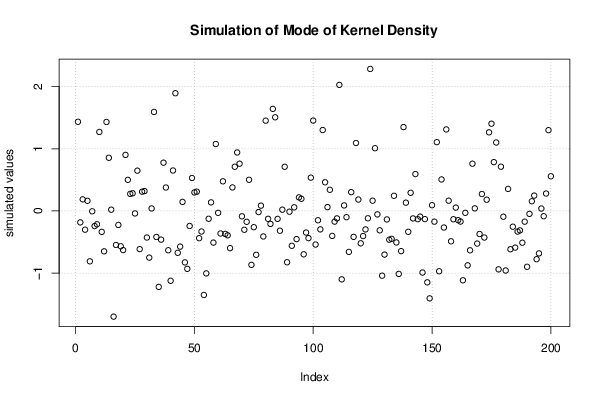
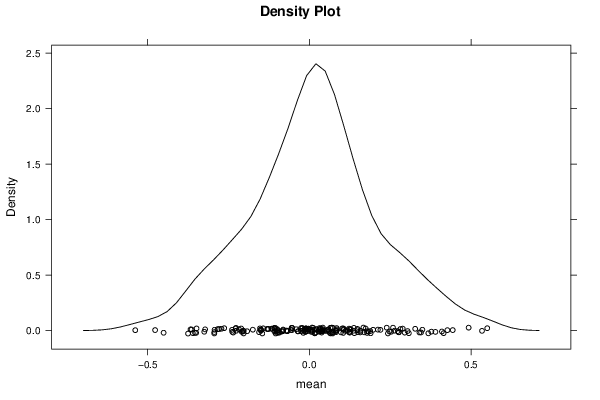
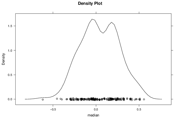
Title produced by software

Bootstrap Plot - Central Tendency

Date of computation

Mon, 15 Dec 2014 20:01:24 +0000

Cite this page as follows

Statistical Computations at FreeStatistics.org, Office for Research Development and Education, URL https://freestatistics.org/blog/index.php?v=date/2014/Dec/15/t1418673705e1dpzl7b0zdu39k.htm/, Retrieved Sun, 19 May 2024 13:34:45 +0000

Statistical Computations at FreeStatistics.org, Office for Research Development and Education, URL https://freestatistics.org/blog/index.php?pk=268968, Retrieved Sun, 19 May 2024 13:34:45 +0000

QR Codes:

Paste this QR Code to cite your computation.

Original text written by user:

IsPrivate?

No (this computation is public)

User-defined keywords

Estimated Impact

Family? (F = Feedback message, R = changed R code, M = changed R Module, P = changed Parameters, D = changed Data)

-     [Central Tendency] [] [2014-11-04 10:08:09] [32b17a345b130fdf5cc88718ed94a974]
-       [Central Tendency] [WS7 3] [2014-11-12 20:26:33] [81f624c2f0b20a2549c93e7c3dccf981]
-    D    [Central Tendency] [] [2014-12-15 16:40:00] [ae96d02647dd9ad9c105f1fa6642e295]
- RM D        [Bootstrap Plot - Central Tendency] [] [2014-12-15 20:01:24] [4ade5e15fc88dfcb6333f94ac70b9a75] [Current]

Feedback Forum

Post a new message

Dataseries X:

Download CSV

Histogram

Boxplots

0.0991579
-0.24856
-0.129539
-5.65751
-6.22954
-0.265554
1.6447
0.434446
-2.27816
-4.98621
-1.59352
-6.75458
-2.16921
-1.12149
-6.5023
-1.78987
-1.12515
-3.72588
-3.33027
-2.89718
-6.88182
0.74249
-2.41856
1.28818
-1.4553
-2.02954
3.04104
0.310134
-3.09352
-1.65385
-4.69425
-1.42222
-3.99352
-3.2928
-2.28987
-2.40595
-2.14563
-0.453851
-3.62954
-0.905954
-6.99718
-1.36921
-0.284001
-2.28987
-0.822221
-1.21327
-1.28987
-5.09352
0.25144
-0.565554
-1.32954
-6.26262
-2.18987
-1.24653
-0.0141772
-2.79718
-7.48766
1.56387
-4.57653
0.210134
-3.72588
-0.172872
-4.97726
2.81013
-3.66628
-3.6045
-1.79718
0.038105
1.63445
-0.793524
-0.886207
-1.49718
-3.93758
2.11981
0.150714
-0.0582362
-0.104501
0.17412
-3.09425
-5.38987
-2.42954
0.534446
-2.18987
-8.56555
-2.88693
-1.32222
-1.88987
-1.2736
-4.13686
0.495499
-0.298636
-7.20157
-3.38182
-4.1619
-5.1332
-4.08987
-5.69352
-1.3045
1.24851
-4.70889
-2.42222
-2.78987
-4.21182
-3.61784
1.36608
-4.65458
0.891114
-8.0619
-6.40157
-3.07287
-1.39352
-1.15515
-8.83693
-0.422221
5.01013
4.76013
3.73372
-0.393524
4.20282
6.10648
2.94542
0.646226
5.82347
1.61086
-2.45824
-0.58548
3.01307
0.221838
5.81013
0.946149
1.41013
3.15648
1.81973
1.61307
-0.542798
-0.439866
4.16379
-4.77816
5.47046
2.91379
-0.720589
4.72485
2.25648
4.56013
3.26013
4.72046
0.510134
1.26013
1.66013
5.35282
-3.12661
2.78071
5.16013
3.85648
1.47778
0.695423
5.6351
2.60648
1.79249
-1.33987
5.36013
2.64908
4.1381
2.7851
7.3551
-2.04352
5.45575
2.10648
2.10209
-1.77222
2.57184
5.07339
1.76608
2.37412
2.37412
4.57412
0.29249
6.33006
2.26013
-4.75222
0.662417
1.22568
6.07412
2.09542
-0.158963
3.10648
4.5168
0.25209
-0.619213
-0.619289
-2.67661
2.27778
-3.29718
5.14176
1.02347
1.76013
1.72339
0.977779
2.06608
3.09542
6.22485
0.509408
0.605749
2.49542
0.174196
1.60648
-3.40019
-0.280266
6.686
4.24778
-1.98621
1.9351
-1.19059
0.880864
3.54916
-0.400842
2.79176
4.89981
-2.03693
2.75282
4.72412
-5.66418
-0.772221
2.79843
6.21013
2.46242
4.1072
2.60648
5.08582
6.05648
5.55575
6.10575
-0.0538508
-0.20751
-3.87816
-8.62222
-0.727257
0.734446
-1.32588
-0.914177
0.324846
-1.75385
1.81013
7.3551
-1.3758
1.60575
4.22111
1.28151
3.17046
0.32412
-1.11117
-0.947183
1.66013
1.89908
0.398431
3.79176
-5.30385
-5.26117
-0.00888631
-5.27222
-2.04352
-0.387583
-3.13987
1.81013
3.56013
0.405749
1.05282
2.61013
3.72778
-2.33255
2.25868
-1.43701
2.04176
4.66013
2.04542
1.51013
3.84843
-4.51034

Summary of computational transaction
Raw Input	view raw input (R code)
Raw Output	view raw output of R engine
Computing time	6 seconds
R Server	'Gertrude Mary Cox' @ cox.wessa.net

\begin{tabular}{lllllllll}
\hline
Summary of computational transaction \tabularnewline
Raw Input & view raw input (R code)  \tabularnewline
Raw Output & view raw output of R engine  \tabularnewline
Computing time & 6 seconds \tabularnewline
R Server & 'Gertrude Mary Cox' @ cox.wessa.net \tabularnewline
\hline
\end{tabular}
%Source: https://freestatistics.org/blog/index.php?pk=268968&T=0

[TABLE]
[ROW][C]Summary of computational transaction[/C][/ROW]
[ROW][C]Raw Input[/C][C]view raw input (R code) [/C][/ROW]
[ROW][C]Raw Output[/C][C]view raw output of R engine [/C][/ROW]
[ROW][C]Computing time[/C][C]6 seconds[/C][/ROW]
[ROW][C]R Server[/C][C]'Gertrude Mary Cox' @ cox.wessa.net[/C][/ROW]
[/TABLE]
Source: https://freestatistics.org/blog/index.php?pk=268968&T=0

Globally Unique Identifier (entire table): ba.freestatistics.org/blog/index.php?pk=268968&T=0

As an alternative you can also use a QR Code:

The GUIDs for individual cells are displayed in the table below:

Summary of computational transaction
Raw Input	view raw input (R code)
Raw Output	view raw output of R engine
Computing time	6 seconds
R Server	'Gertrude Mary Cox' @ cox.wessa.net

Estimation Results of Bootstrap
statistic	P1	P5	Q1	Estimate	Q3	P95	P99	S.D.	IQR
mean	-0.45101	-0.32612	-0.10489	-1.4968e-07	0.12477	0.35039	0.49303	0.19837	0.22966
median	-0.41195	-0.29168	-0.10553	0.014609	0.19362	0.40628	0.51013	0.2205	0.29914
midrange	-1.2534	-1.0755	-0.74092	-0.74092	-0.63356	-0.3534	0.076765	0.22342	0.10736
mode	-6.27	-4.236	-2.0435	0.61742	2.2345	5.0734	7.3551	2.8571	4.278
mode k.dens	-1.3534	-1.0063	-0.47017	-0.080049	0.30343	1.4046	1.8954	0.70602	0.7736

\begin{tabular}{lllllllll}
\hline
Estimation Results of Bootstrap \tabularnewline
statistic & P1 & P5 & Q1 & Estimate & Q3 & P95 & P99 & S.D. & IQR \tabularnewline
mean & -0.45101 & -0.32612 & -0.10489 & -1.4968e-07 & 0.12477 & 0.35039 & 0.49303 & 0.19837 & 0.22966 \tabularnewline
median & -0.41195 & -0.29168 & -0.10553 & 0.014609 & 0.19362 & 0.40628 & 0.51013 & 0.2205 & 0.29914 \tabularnewline
midrange & -1.2534 & -1.0755 & -0.74092 & -0.74092 & -0.63356 & -0.3534 & 0.076765 & 0.22342 & 0.10736 \tabularnewline
mode & -6.27 & -4.236 & -2.0435 & 0.61742 & 2.2345 & 5.0734 & 7.3551 & 2.8571 & 4.278 \tabularnewline
mode k.dens & -1.3534 & -1.0063 & -0.47017 & -0.080049 & 0.30343 & 1.4046 & 1.8954 & 0.70602 & 0.7736 \tabularnewline
\hline
\end{tabular}
%Source: https://freestatistics.org/blog/index.php?pk=268968&T=1

[TABLE]
[ROW][C]Estimation Results of Bootstrap[/C][/ROW]
[ROW][C]statistic[/C][C]P1[/C][C]P5[/C][C]Q1[/C][C]Estimate[/C][C]Q3[/C][C]P95[/C][C]P99[/C][C]S.D.[/C][C]IQR[/C][/ROW]
[ROW][C]mean[/C][C]-0.45101[/C][C]-0.32612[/C][C]-0.10489[/C][C]-1.4968e-07[/C][C]0.12477[/C][C]0.35039[/C][C]0.49303[/C][C]0.19837[/C][C]0.22966[/C][/ROW]
[ROW][C]median[/C][C]-0.41195[/C][C]-0.29168[/C][C]-0.10553[/C][C]0.014609[/C][C]0.19362[/C][C]0.40628[/C][C]0.51013[/C][C]0.2205[/C][C]0.29914[/C][/ROW]
[ROW][C]midrange[/C][C]-1.2534[/C][C]-1.0755[/C][C]-0.74092[/C][C]-0.74092[/C][C]-0.63356[/C][C]-0.3534[/C][C]0.076765[/C][C]0.22342[/C][C]0.10736[/C][/ROW]
[ROW][C]mode[/C][C]-6.27[/C][C]-4.236[/C][C]-2.0435[/C][C]0.61742[/C][C]2.2345[/C][C]5.0734[/C][C]7.3551[/C][C]2.8571[/C][C]4.278[/C][/ROW]
[ROW][C]mode k.dens[/C][C]-1.3534[/C][C]-1.0063[/C][C]-0.47017[/C][C]-0.080049[/C][C]0.30343[/C][C]1.4046[/C][C]1.8954[/C][C]0.70602[/C][C]0.7736[/C][/ROW]
[/TABLE]
Source: https://freestatistics.org/blog/index.php?pk=268968&T=1

Globally Unique Identifier (entire table): ba.freestatistics.org/blog/index.php?pk=268968&T=1

As an alternative you can also use a QR Code:

The GUIDs for individual cells are displayed in the table below:

Estimation Results of Bootstrap
statistic	P1	P5	Q1	Estimate	Q3	P95	P99	S.D.	IQR
mean	-0.45101	-0.32612	-0.10489	-1.4968e-07	0.12477	0.35039	0.49303	0.19837	0.22966
median	-0.41195	-0.29168	-0.10553	0.014609	0.19362	0.40628	0.51013	0.2205	0.29914
midrange	-1.2534	-1.0755	-0.74092	-0.74092	-0.63356	-0.3534	0.076765	0.22342	0.10736
mode	-6.27	-4.236	-2.0435	0.61742	2.2345	5.0734	7.3551	2.8571	4.278
mode k.dens	-1.3534	-1.0063	-0.47017	-0.080049	0.30343	1.4046	1.8954	0.70602	0.7736

Figure 1

PNG link

Postscript link

PDF link

Figure 2

PNG link

Postscript link

PDF link

Figure 3

PNG link

Postscript link

PDF link

Figure 4

PNG link

Postscript link

PDF link

Figure 5

PNG link

Postscript link

PDF link

Figure 6

PNG link

Postscript link

PDF link

Figure 7

PNG link

Postscript link

PDF link

Figure 8

PNG link

Postscript link

PDF link

Figure 9

PNG link

Postscript link

PDF link

Figure 10

PNG link

Postscript link

PDF link

Figure 11

PNG link

Postscript link

PDF link

Parameters (Session):

Parameters (R input):

par1 = 200 ; par2 = 5 ; par3 = 0 ; par4 = P1 P5 Q1 Q3 P95 P99 ;

R code (references can be found in the software module):

par1 <- as.numeric(par1)
par2 <- as.numeric(par2)
if (par3 == '0') bw <- NULL
if (par3 != '0') bw <- as.numeric(par3)
if (par1 < 10) par1 = 10
if (par1 > 5000) par1 = 5000
library(modeest)
library(lattice)
library(boot)
boot.stat <- function(s,i)
{
s.mean <- mean(s[i])
s.median <- median(s[i])
s.midrange <- (max(s[i]) + min(s[i])) / 2
s.mode <- mlv(s[i], method='mfv')$M
s.kernelmode <- mlv(s[i], method='kernel', bw=bw)$M
c(s.mean, s.median, s.midrange, s.mode, s.kernelmode)
}
(r <- boot(x,boot.stat, R=par1, stype='i'))
bitmap(file='plot1.png')
plot(r$t[,1],type='p',ylab='simulated values',main='Simulation of Mean')
grid()
dev.off()
bitmap(file='plot2.png')
plot(r$t[,2],type='p',ylab='simulated values',main='Simulation of Median')
grid()
dev.off()
bitmap(file='plot3.png')
plot(r$t[,3],type='p',ylab='simulated values',main='Simulation of Midrange')
grid()
dev.off()
bitmap(file='plot7.png')
plot(r$t[,4],type='p',ylab='simulated values',main='Simulation of Mode')
grid()
dev.off()
bitmap(file='plot8.png')
plot(r$t[,5],type='p',ylab='simulated values',main='Simulation of Mode of Kernel Density')
grid()
dev.off()
bitmap(file='plot4.png')
densityplot(~r$t[,1],col='black',main='Density Plot',xlab='mean')
dev.off()
bitmap(file='plot5.png')
densityplot(~r$t[,2],col='black',main='Density Plot',xlab='median')
dev.off()
bitmap(file='plot6.png')
densityplot(~r$t[,3],col='black',main='Density Plot',xlab='midrange')
dev.off()
bitmap(file='plot9.png')
densityplot(~r$t[,4],col='black',main='Density Plot',xlab='mode')
dev.off()
bitmap(file='plot10.png')
densityplot(~r$t[,5],col='black',main='Density Plot',xlab='mode of kernel dens.')
dev.off()
z <- data.frame(cbind(r$t[,1],r$t[,2],r$t[,3],r$t[,4],r$t[,5]))
colnames(z) <- list('mean','median','midrange','mode','mode k.dens')
bitmap(file='plot11.png')
boxplot(z,notch=TRUE,ylab='simulated values',main='Bootstrap Simulation - Central Tendency')
grid()
dev.off()
load(file='createtable')
a<-table.start()
a<-table.row.start(a)
a<-table.element(a,'Estimation Results of Bootstrap',10,TRUE)
a<-table.row.end(a)
if (par4 == 'P1 P5 Q1 Q3 P95 P99') {
myq.1 <- 0.01
myq.2 <- 0.05
myq.3 <- 0.95
myq.4 <- 0.99
myl.1 <- 'P1'
myl.2 <- 'P5'
myl.3 <- 'P95'
myl.4 <- 'P99'
}
if (par4 == 'P0.5 P2.5 Q1 Q3 P97.5 P99.5') {
myq.1 <- 0.005
myq.2 <- 0.025
myq.3 <- 0.975
myq.4 <- 0.995
myl.1 <- 'P0.5'
myl.2 <- 'P2.5'
myl.3 <- 'P97.5'
myl.4 <- 'P99.5'
}
if (par4 == 'P10 P20 Q1 Q3 P80 P90') {
myq.1 <- 0.10
myq.2 <- 0.20
myq.3 <- 0.80
myq.4 <- 0.90
myl.1 <- 'P10'
myl.2 <- 'P20'
myl.3 <- 'P80'
myl.4 <- 'P90'
}
a<-table.row.start(a)
a<-table.element(a,'statistic',header=TRUE)
a<-table.element(a,myl.1,header=TRUE)
a<-table.element(a,myl.2,header=TRUE)
a<-table.element(a,'Q1',header=TRUE)
a<-table.element(a,'Estimate',header=TRUE)
a<-table.element(a,'Q3',header=TRUE)
a<-table.element(a,myl.3,header=TRUE)
a<-table.element(a,myl.4,header=TRUE)
a<-table.element(a,'S.D.',header=TRUE)
a<-table.element(a,'IQR',header=TRUE)
a<-table.row.end(a)
a<-table.row.start(a)
a<-table.element(a,'mean',header=TRUE)
q1 <- quantile(r$t[,1],0.25)[[1]]
q3 <- quantile(r$t[,1],0.75)[[1]]
p01 <- quantile(r$t[,1],myq.1)[[1]]
p05 <- quantile(r$t[,1],myq.2)[[1]]
p95 <- quantile(r$t[,1],myq.3)[[1]]
p99 <- quantile(r$t[,1],myq.4)[[1]]
a<-table.element(a,signif(p01,par2))
a<-table.element(a,signif(p05,par2))
a<-table.element(a,signif(q1,par2))
a<-table.element(a,signif(r$t0[1],par2))
a<-table.element(a,signif(q3,par2))
a<-table.element(a,signif(p95,par2))
a<-table.element(a,signif(p99,par2))
a<-table.element( a,signif( sqrt(var(r$t[,1])),par2 ) )
a<-table.element(a,signif(q3-q1,par2))
a<-table.row.end(a)
a<-table.row.start(a)
a<-table.element(a,'median',header=TRUE)
q1 <- quantile(r$t[,2],0.25)[[1]]
q3 <- quantile(r$t[,2],0.75)[[1]]
p01 <- quantile(r$t[,2],myq.1)[[1]]
p05 <- quantile(r$t[,2],myq.2)[[1]]
p95 <- quantile(r$t[,2],myq.3)[[1]]
p99 <- quantile(r$t[,2],myq.4)[[1]]
a<-table.element(a,signif(p01,par2))
a<-table.element(a,signif(p05,par2))
a<-table.element(a,signif(q1,par2))
a<-table.element(a,signif(r$t0[2],par2))
a<-table.element(a,signif(q3,par2))
a<-table.element(a,signif(p95,par2))
a<-table.element(a,signif(p99,par2))
a<-table.element(a,signif(sqrt(var(r$t[,2])),par2))
a<-table.element(a,signif(q3-q1,par2))
a<-table.row.end(a)
a<-table.row.start(a)
a<-table.element(a,'midrange',header=TRUE)
q1 <- quantile(r$t[,3],0.25)[[1]]
q3 <- quantile(r$t[,3],0.75)[[1]]
p01 <- quantile(r$t[,3],myq.1)[[1]]
p05 <- quantile(r$t[,3],myq.2)[[1]]
p95 <- quantile(r$t[,3],myq.3)[[1]]
p99 <- quantile(r$t[,3],myq.4)[[1]]
a<-table.element(a,signif(p01,par2))
a<-table.element(a,signif(p05,par2))
a<-table.element(a,signif(q1,par2))
a<-table.element(a,signif(r$t0[3],par2))
a<-table.element(a,signif(q3,par2))
a<-table.element(a,signif(p95,par2))
a<-table.element(a,signif(p99,par2))
a<-table.element(a,signif(sqrt(var(r$t[,3])),par2))
a<-table.element(a,signif(q3-q1,par2))
a<-table.row.end(a)
a<-table.row.start(a)
a<-table.element(a,'mode',header=TRUE)
q1 <- quantile(r$t[,4],0.25)[[1]]
q3 <- quantile(r$t[,4],0.75)[[1]]
p01 <- quantile(r$t[,4],myq.1)[[1]]
p05 <- quantile(r$t[,4],myq.2)[[1]]
p95 <- quantile(r$t[,4],myq.3)[[1]]
p99 <- quantile(r$t[,4],myq.4)[[1]]
a<-table.element(a,signif(p01,par2))
a<-table.element(a,signif(p05,par2))
a<-table.element(a,signif(q1,par2))
a<-table.element(a,signif(r$t0[4],par2))
a<-table.element(a,signif(q3,par2))
a<-table.element(a,signif(p95,par2))
a<-table.element(a,signif(p99,par2))
a<-table.element(a,signif(sqrt(var(r$t[,4])),par2))
a<-table.element(a,signif(q3-q1,par2))
a<-table.row.end(a)
a<-table.row.start(a)
a<-table.element(a,'mode k.dens',header=TRUE)
q1 <- quantile(r$t[,5],0.25)[[1]]
q3 <- quantile(r$t[,5],0.75)[[1]]
p01 <- quantile(r$t[,5],myq.1)[[1]]
p05 <- quantile(r$t[,5],myq.2)[[1]]
p95 <- quantile(r$t[,5],myq.3)[[1]]
p99 <- quantile(r$t[,5],myq.4)[[1]]
a<-table.element(a,signif(p01,par2))
a<-table.element(a,signif(p05,par2))
a<-table.element(a,signif(q1,par2))
a<-table.element(a,signif(r$t0[5],par2))
a<-table.element(a,signif(q3,par2))
a<-table.element(a,signif(p95,par2))
a<-table.element(a,signif(p99,par2))
a<-table.element(a,signif(sqrt(var(r$t[,5])),par2))
a<-table.element(a,signif(q3-q1,par2))
a<-table.row.end(a)
a<-table.end(a)
table.save(a,file='mytable.tab')

Free Statistics

Description of Statistical Computation

Tree of Dependent Computations

Dataset

Tables (Output of Computation)

Figures (Output of Computation)

Input Parameters & R Code