Free Statistics
of Irreproducible Research!
Description of Statistical Computation | |||||||||||||||||||||||||||||||||||||||||||||||||||||||||||||||||||||||||||||||||||||||||||||||||||||
|---|---|---|---|---|---|---|---|---|---|---|---|---|---|---|---|---|---|---|---|---|---|---|---|---|---|---|---|---|---|---|---|---|---|---|---|---|---|---|---|---|---|---|---|---|---|---|---|---|---|---|---|---|---|---|---|---|---|---|---|---|---|---|---|---|---|---|---|---|---|---|---|---|---|---|---|---|---|---|---|---|---|---|---|---|---|---|---|---|---|---|---|---|---|---|---|---|---|---|---|---|---|
| Author's title | |||||||||||||||||||||||||||||||||||||||||||||||||||||||||||||||||||||||||||||||||||||||||||||||||||||
| Author | *The author of this computation has been verified* | ||||||||||||||||||||||||||||||||||||||||||||||||||||||||||||||||||||||||||||||||||||||||||||||||||||
| R Software Module | rwasp_notchedbox1.wasp | ||||||||||||||||||||||||||||||||||||||||||||||||||||||||||||||||||||||||||||||||||||||||||||||||||||
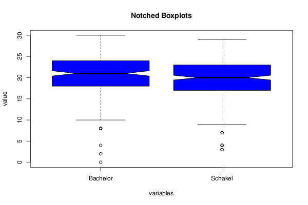
| Title produced by software | Notched Boxplots | ||||||||||||||||||||||||||||||||||||||||||||||||||||||||||||||||||||||||||||||||||||||||||||||||||||
| Date of computation | Mon, 15 Dec 2014 14:03:29 +0000 | ||||||||||||||||||||||||||||||||||||||||||||||||||||||||||||||||||||||||||||||||||||||||||||||||||||
| Cite this page as follows | Statistical Computations at FreeStatistics.org, Office for Research Development and Education, URL https://freestatistics.org/blog/index.php?v=date/2014/Dec/15/t141865229196875r7bazfntlr.htm/, Retrieved Sun, 19 May 2024 16:10:32 +0000 | ||||||||||||||||||||||||||||||||||||||||||||||||||||||||||||||||||||||||||||||||||||||||||||||||||||
| Statistical Computations at FreeStatistics.org, Office for Research Development and Education, URL https://freestatistics.org/blog/index.php?pk=268434, Retrieved Sun, 19 May 2024 16:10:32 +0000 | |||||||||||||||||||||||||||||||||||||||||||||||||||||||||||||||||||||||||||||||||||||||||||||||||||||
| QR Codes: | |||||||||||||||||||||||||||||||||||||||||||||||||||||||||||||||||||||||||||||||||||||||||||||||||||||
|
| |||||||||||||||||||||||||||||||||||||||||||||||||||||||||||||||||||||||||||||||||||||||||||||||||||||
| Original text written by user: | |||||||||||||||||||||||||||||||||||||||||||||||||||||||||||||||||||||||||||||||||||||||||||||||||||||
| IsPrivate? | No (this computation is public) | ||||||||||||||||||||||||||||||||||||||||||||||||||||||||||||||||||||||||||||||||||||||||||||||||||||
| User-defined keywords | |||||||||||||||||||||||||||||||||||||||||||||||||||||||||||||||||||||||||||||||||||||||||||||||||||||
| Estimated Impact | 81 | ||||||||||||||||||||||||||||||||||||||||||||||||||||||||||||||||||||||||||||||||||||||||||||||||||||
Tree of Dependent Computations | |||||||||||||||||||||||||||||||||||||||||||||||||||||||||||||||||||||||||||||||||||||||||||||||||||||
| Family? (F = Feedback message, R = changed R code, M = changed R Module, P = changed Parameters, D = changed Data) | |||||||||||||||||||||||||||||||||||||||||||||||||||||||||||||||||||||||||||||||||||||||||||||||||||||
| - [Maximum-likelihood Fitting - Normal Distribution] [Intrinsic Motivat...] [2010-10-12 11:57:21] [b98453cac15ba1066b407e146608df68] - RMP [Maximum-likelihood Fitting - Normal Distribution] [] [2014-10-14 18:01:50] [32b17a345b130fdf5cc88718ed94a974] - MP [Maximum-likelihood Fitting - Normal Distribution] [] [2014-10-15 14:22:38] [bcf5edf18529a33bd1494456d2c6cb9a] - RMPD [Notched Boxplots] [] [2014-12-15 14:03:29] [023a69c6c348bca0f1811b046758af62] [Current] | |||||||||||||||||||||||||||||||||||||||||||||||||||||||||||||||||||||||||||||||||||||||||||||||||||||
| Feedback Forum | |||||||||||||||||||||||||||||||||||||||||||||||||||||||||||||||||||||||||||||||||||||||||||||||||||||
Post a new message | |||||||||||||||||||||||||||||||||||||||||||||||||||||||||||||||||||||||||||||||||||||||||||||||||||||
Dataset | |||||||||||||||||||||||||||||||||||||||||||||||||||||||||||||||||||||||||||||||||||||||||||||||||||||
| Dataseries X: | |||||||||||||||||||||||||||||||||||||||||||||||||||||||||||||||||||||||||||||||||||||||||||||||||||||
15 21 20 26 21 22 8 20 19 19 22 18 12 21 22 15 12 21 22 16 10 16 22 19 24 10 18 26 22 23 20 16 19 23 11 21 8 19 15 18 18 25 18 19 19 14 30 16 27 20 18 23 28 18 27 18 28 19 21 22 22 14 20 23 23 20 18 13 18 16 25 7 25 17 25 19 24 23 13 19 17 16 4 20 16 25 21 17 20 12 22 24 0 14 18 18 29 19 15 16 22 19 22 4 17 20 27 24 15 17 26 22 18 19 27 22 17 23 19 23 13 24 16 7 2 19 26 19 22 16 18 19 21 24 24 16 17 16 20 26 21 18 21 19 16 19 15 16 21 16 18 16 22 20 23 15 22 22 20 16 27 11 20 16 21 15 26 16 18 18 16 25 20 22 18 17 16 22 10 23 23 13 23 19 19 15 17 20 26 15 20 20 24 13 20 24 16 20 22 22 19 26 15 25 12 23 15 14 18 24 18 13 12 23 28 22 21 26 30 16 14 11 18 19 19 25 25 19 23 22 17 14 21 22 29 18 20 23 23 12 24 22 20 21 23 19 17 22 21 15 20 20 20 20 19 16 26 23 23 18 24 25 21 9 21 23 8 25 17 25 20 18 19 23 17 21 24 22 20 23 25 23 20 24 21 24 22 15 25 19 28 18 29 27 20 13 20 28 19 19 19 19 26 17 10 26 17 28 30 24 22 23 23 22 16 21 18 25 25 27 18 23 24 23 23 19 24 15 15 20 20 16 26 25 23 25 23 19 22 16 15 19 22 19 10 23 20 21 23 19 27 20 23 3 25 23 20 15 24 24 19 24 24 24 19 28 21 23 27 25 20 25 17 20 21 25 18 23 24 20 27 16 20 23 25 11 21 23 25 29 20 16 27 23 18 20 26 4 18 24 21 16 18 3 25 23 20 20 23 19 22 24 18 27 25 22 22 17 14 23 26 28 15 29 21 21 20 20 22 28 20 26 26 20 20 23 15 24 25 21 20 16 27 21 17 28 22 23 24 29 22 18 23 22 20 14 22 15 27 15 24 20 25 21 19 17 24 20 22 24 18 28 NA 20 NA 27 NA 22 NA 24 NA 18 NA 19 NA 23 NA 23 NA 19 NA 25 NA 24 NA 27 NA 16 NA 15 NA 27 NA 21 NA 16 NA 22 NA 17 NA 23 NA 14 NA 24 NA 21 NA 16 NA 19 NA 16 NA 11 NA 23 NA 27 NA 23 NA 24 NA 22 NA 26 NA 19 NA 19 NA 20 NA 16 NA 22 NA 21 NA 26 NA 23 NA 21 NA 26 NA 27 NA 17 NA 22 NA 19 NA 20 NA 26 | |||||||||||||||||||||||||||||||||||||||||||||||||||||||||||||||||||||||||||||||||||||||||||||||||||||
Tables (Output of Computation) | |||||||||||||||||||||||||||||||||||||||||||||||||||||||||||||||||||||||||||||||||||||||||||||||||||||
| |||||||||||||||||||||||||||||||||||||||||||||||||||||||||||||||||||||||||||||||||||||||||||||||||||||
Figures (Output of Computation) | |||||||||||||||||||||||||||||||||||||||||||||||||||||||||||||||||||||||||||||||||||||||||||||||||||||
Input Parameters & R Code | |||||||||||||||||||||||||||||||||||||||||||||||||||||||||||||||||||||||||||||||||||||||||||||||||||||
| Parameters (Session): | |||||||||||||||||||||||||||||||||||||||||||||||||||||||||||||||||||||||||||||||||||||||||||||||||||||
| par1 = grey ; | |||||||||||||||||||||||||||||||||||||||||||||||||||||||||||||||||||||||||||||||||||||||||||||||||||||
| Parameters (R input): | |||||||||||||||||||||||||||||||||||||||||||||||||||||||||||||||||||||||||||||||||||||||||||||||||||||
| par1 = blue ; | |||||||||||||||||||||||||||||||||||||||||||||||||||||||||||||||||||||||||||||||||||||||||||||||||||||
| R code (references can be found in the software module): | |||||||||||||||||||||||||||||||||||||||||||||||||||||||||||||||||||||||||||||||||||||||||||||||||||||
z <- as.data.frame(t(y)) | |||||||||||||||||||||||||||||||||||||||||||||||||||||||||||||||||||||||||||||||||||||||||||||||||||||