Repository of Reproducible Computations

Free Statistics

of Irreproducible Research!

Author's title

Author

*The author of this computation has been verified*

R Software Module

rwasp_meanversusmedian.wasp

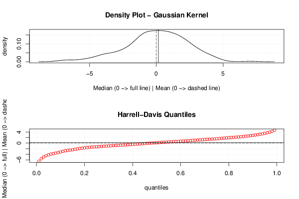
Title produced by software

Mean versus Median

Date of computation

Wed, 10 Dec 2014 15:28:53 +0000

Cite this page as follows

Statistical Computations at FreeStatistics.org, Office for Research Development and Education, URL https://freestatistics.org/blog/index.php?v=date/2014/Dec/10/t1418225402kx1tg5duwhngbw2.htm/, Retrieved Sun, 19 May 2024 14:58:01 +0000

Statistical Computations at FreeStatistics.org, Office for Research Development and Education, URL https://freestatistics.org/blog/index.php?pk=265383, Retrieved Sun, 19 May 2024 14:58:01 +0000

QR Codes:

Paste this QR Code to cite your computation.

Original text written by user:

IsPrivate?

No (this computation is public)

User-defined keywords

Estimated Impact

Family? (F = Feedback message, R = changed R code, M = changed R Module, P = changed Parameters, D = changed Data)

-       [Mean versus Median] [] [2014-12-10 15:28:53] [e4f070d9a53956de258aedfd2fe319be] [Current]

Feedback Forum

Post a new message

Dataseries X:

Download CSV

Histogram

Boxplots

0.345006
1.15138
0.632995
-3.7032
-4.00853
-1.02644
3.46231
4.17772
0.445131
-4.11427
-0.334685
-4.57871
1.48896
-0.608659
-0.619642
2.1307
0.110907
-1.1539
-2.03183
0.481007
-4.30006
3.12242
-3.73052
0.979097
1.20476
-3.70508
3.92608
3.43759
-1.25958
0.197172
-0.417328
0.330198
-1.09907
-1.7785
2.09027
1.49051
-0.813218
2.02382
-2.57638
-0.312824
-4.19186
0.0373626
1.61194
-0.82974
4.38674
-2.27504
2.87627
-1.51329
3.31255
2.59552
0.955112
-0.226644
-0.231719
0.0446019
3.54234
0.229488
-5.52552
4.52165
-0.161258
2.89446
-2.80165
0.112315
-0.943851
2.46693
-3.71833
0.598926
-1.47701
-0.978677
1.88307
1.19956
-0.612326
0.624379
-0.657413
3.92001
1.78334
1.24034
1.55312
1.17396
0.821636
-1.60267
-0.17704
2.59874
0.884215
-5.2848
-0.650795
1.66128
2.30977
2.11941
-1.74422
1.1313
4.00354
-4.67799
-1.52349
-1.08668
-2.41814
-2.35028
-3.90459
1.57116
3.01709
-2.50554
2.26411
-0.00213422
-0.850237
-1.31838
4.38016
-1.50217
3.54948
-5.03989
-1.9675
-1.17735
0.284271
0.712484
-6.95062
1.01476
2.78537
2.01994
0.213286
0.365394
-1.30299
2.22056
0.478691
0.512394
1.72538
4.20732
-2.70796
-0.854175
1.42083
0.495151
3.03705
0.599904
0.628718
-0.425919
1.02859
1.53412
-0.1706
0.0981743
2.81253
-1.50298
2.32932
2.03915
-0.826478
1.47023
0.965417
3.44802
0.0677638
1.18224
-0.675474
-0.0347173
-0.228656
1.54925
-6.33165
1.96989
2.11003
-0.747912
1.24831
-0.126449
2.43329
1.033
-1.56978
-2.436
2.05592
2.20024
-0.438765
7.00785
1.1741
-0.344619
2.25716
0.532103
-0.349491
-2.4046
1.52639
2.69028
-2.00594
-1.01881
-0.958034
3.01803
-0.89783
2.37466
-1.36717
-4.04062
-1.46298
-2.38194
3.07292
0.310059
-2.8529
0.526583
1.81057
-2.52733
-3.60994
0.442267
-2.77948
1.65781
-3.68493
3.24545
-1.12272
1.30223
-1.55108
0.560124
0.764836
0.688621
0.774914
0.207235
-1.94888
-0.123195
-1.50622
0.914723
-0.536938
0.152812
3.75825
2.14345
-0.767506
-0.125028
-1.60226
-1.024
-0.191978
-0.728723
1.61705
1.53029
-1.2036
-0.736613
2.31377
-3.82648
-1.98916
1.46859
2.62574
2.70082
1.42321
1.75542
4.3433
2.93969
2.54086
3.38229
-0.588523
-3.39632
-2.59544
-6.76343
-0.748894
-0.831369
-0.399049
-0.865302
-1.18534
-1.44527
0.241105
2.02872
-3.42284
-0.289255
0.759704
0.163727
0.953235
-1.17571
-3.39457
-1.21656
0.584745
2.11272
-2.67681
0.974455
-4.90915
-5.44278
-2.30565
-6.90284
-1.17766
-2.53571
-3.29379
0.764595
1.70931
0.274045
-0.814493
1.03814
1.35389
-1.42654
-0.0346729
-0.594272
1.52455
2.00008
0.571877
-0.631742
0.90847
-2.75195

Summary of computational transaction
Raw Input	view raw input (R code)
Raw Output	view raw output of R engine
Computing time	1 seconds
R Server	'Sir Maurice George Kendall' @ kendall.wessa.net

\begin{tabular}{lllllllll}
\hline
Summary of computational transaction \tabularnewline
Raw Input & view raw input (R code)  \tabularnewline
Raw Output & view raw output of R engine  \tabularnewline
Computing time & 1 seconds \tabularnewline
R Server & 'Sir Maurice George Kendall' @ kendall.wessa.net \tabularnewline
\hline
\end{tabular}
%Source: https://freestatistics.org/blog/index.php?pk=265383&T=0

[TABLE]
[ROW][C]Summary of computational transaction[/C][/ROW]
[ROW][C]Raw Input[/C][C]view raw input (R code) [/C][/ROW]
[ROW][C]Raw Output[/C][C]view raw output of R engine [/C][/ROW]
[ROW][C]Computing time[/C][C]1 seconds[/C][/ROW]
[ROW][C]R Server[/C][C]'Sir Maurice George Kendall' @ kendall.wessa.net[/C][/ROW]
[/TABLE]
Source: https://freestatistics.org/blog/index.php?pk=265383&T=0

Globally Unique Identifier (entire table): ba.freestatistics.org/blog/index.php?pk=265383&T=0

As an alternative you can also use a QR Code:

The GUIDs for individual cells are displayed in the table below:

Summary of computational transaction
Raw Input	view raw input (R code)
Raw Output	view raw output of R engine
Computing time	1 seconds
R Server	'Sir Maurice George Kendall' @ kendall.wessa.net

Median versus Mean
mean	6.8992805751302e-08
median	0.1582695

\begin{tabular}{lllllllll}
\hline
Median versus Mean \tabularnewline
mean & 6.8992805751302e-08 \tabularnewline
median & 0.1582695 \tabularnewline
\hline
\end{tabular}
%Source: https://freestatistics.org/blog/index.php?pk=265383&T=1

[TABLE]
[ROW][C]Median versus Mean[/C][/ROW]
[ROW][C]mean[/C][C]6.8992805751302e-08[/C][/ROW]
[ROW][C]median[/C][C]0.1582695[/C][/ROW]
[/TABLE]
Source: https://freestatistics.org/blog/index.php?pk=265383&T=1

Globally Unique Identifier (entire table): ba.freestatistics.org/blog/index.php?pk=265383&T=1

As an alternative you can also use a QR Code:

The GUIDs for individual cells are displayed in the table below:

Median versus Mean
mean	6.8992805751302e-08
median	0.1582695

Figure 1

PNG link

Postscript link

PDF link

Parameters (Session):

Parameters (R input):

R code (references can be found in the software module):

library(Hmisc)
m <- mean(x)
e <- median(x)
bitmap(file='test1.png')
op <- par(mfrow=c(2,1))
mydensity1 <- density(x,kernel='gaussian',na.rm=TRUE)
plot(mydensity1,main='Density Plot - Gaussian Kernel',xlab='Median (0 -> full line) | Mean (0 -> dashed line)',ylab='density')
abline(v=e,lty=1)
abline(v=m,lty=5)
grid()
myseq <- seq(0.01, 0.99, 0.01)
hd <- hdquantile(x, probs = myseq, se = TRUE, na.rm = FALSE, names = TRUE, weights=FALSE)
plot(myseq,hd,col=2,main='Harrell-Davis Quantiles',xlab='quantiles',ylab='Median (0 -> full) | Mean (0 -> dashed)')
abline(h=m,lty=5)
abline(h=e,lty=1)
grid()
par(op)
dev.off()
load(file='createtable')
a<-table.start()
a<-table.row.start(a)
a<-table.element(a,'Median versus Mean',2,TRUE)
a<-table.row.end(a)
a<-table.row.start(a)
a<-table.element(a,'mean',header=TRUE)
a<-table.element(a,mean(x))
a<-table.row.end(a)
a<-table.row.start(a)
a<-table.element(a,'median',header=TRUE)
a<-table.element(a,median(x))
a<-table.row.end(a)
a<-table.end(a)
table.save(a,file='mytable.tab')

Free Statistics

Description of Statistical Computation

Tree of Dependent Computations

Dataset

Tables (Output of Computation)

Figures (Output of Computation)

Input Parameters & R Code