Repository of Reproducible Computations

Free Statistics

of Irreproducible Research!

Author's title

Author

*The author of this computation has been verified*

R Software Module

rwasp_notchedbox1.wasp

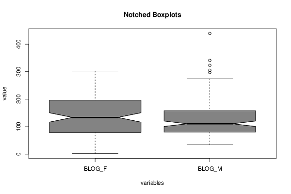
Title produced by software

Notched Boxplots

Date of computation

Wed, 10 Dec 2014 15:26:58 +0000

Cite this page as follows

Statistical Computations at FreeStatistics.org, Office for Research Development and Education, URL https://freestatistics.org/blog/index.php?v=date/2014/Dec/10/t1418225231yn7i5nai6be1feq.htm/, Retrieved Sun, 19 May 2024 14:36:01 +0000

Statistical Computations at FreeStatistics.org, Office for Research Development and Education, URL https://freestatistics.org/blog/index.php?pk=265375, Retrieved Sun, 19 May 2024 14:36:01 +0000

QR Codes:

Paste this QR Code to cite your computation.

Original text written by user:

IsPrivate?

No (this computation is public)

User-defined keywords

Estimated Impact

Family? (F = Feedback message, R = changed R code, M = changed R Module, P = changed Parameters, D = changed Data)

-       [Notched Boxplots] [] [2014-12-10 15:26:58] [fbbeb95c33c8ff026e5ecae513ae1a4b] [Current]
- R       [Notched Boxplots] [] [2014-12-10 18:53:21] [a30ebaf79f34e9d2b1bcdd5006125d11] 

Feedback Forum

Post a new message

Dataseries X:

Download CSV

Histogram

Boxplots

96	NA
NA	70
88	NA
NA	114
NA	69
NA	176
114	NA
NA	121
NA	110
NA	158
NA	116
NA	181
NA	77
141	NA
35	NA
80	NA
NA	152
97	NA
NA	99
84	NA
NA	68
NA	101
107	NA
NA	88
NA	112
NA	171
NA	137
77	NA
NA	66
93	NA
105	NA
131	NA
NA	102
NA	161
NA	120
NA	127
77	NA
NA	108
NA	85
168	NA
NA	48
NA	152
NA	75
NA	107
NA	62
121	NA
NA	124
NA	72
40	NA
NA	58
NA	97
NA	88
NA	126
NA	104
NA	148
NA	146
80	NA
NA	97
25	NA
NA	99
NA	118
58	NA
63	NA
NA	139
50	NA
NA	60
152	NA
NA	142
NA	94
66	NA
127	NA
67	NA
90	NA
NA	75
128	NA
146	NA
NA	69
186	NA
81	NA
NA	85
54	NA
46	NA
106	NA
NA	34
60	NA
NA	95
NA	57
62	NA
36	NA
56	NA
NA	54
NA	64
NA	76
98	NA
NA	88
35	NA
NA	102
NA	61
NA	80
NA	49
NA	78
90	NA
NA	45
NA	55
NA	96
43	NA
52	NA
60	NA
54	NA
51	NA
51	NA
NA	38
NA	41
NA	146
NA	182
NA	192
263	NA
NA	35
NA	439
214	NA
NA	341
58	NA
292	NA
NA	85
NA	200
NA	158
NA	199
NA	297
NA	227
NA	108
NA	86
302	NA
NA	148
NA	178
NA	120
NA	207
NA	157
NA	128
296	NA
NA	323
NA	79
NA	70
NA	146
NA	246
196	NA
199	NA
NA	127
153	NA
299	NA
NA	228
190	NA
NA	180
NA	212
269	NA
NA	130
NA	179
NA	243
190	NA
299	NA
121	NA
137	NA
NA	305
157	NA
NA	96
183	NA
NA	52
238	NA
NA	40
226	NA
190	NA
NA	214
145	NA
NA	119
NA	222
NA	222
NA	159
NA	165
249	NA
NA	125
122	NA
186	NA
148	NA
NA	274
172	NA
NA	84
168	NA
102	NA
106	NA
2	NA
NA	139
NA	95
NA	130
NA	72
141	NA
113	NA
NA	206
268	NA
175	NA
77	NA
125	NA
NA	255
NA	111
132	NA
211	NA
NA	92
76	NA
NA	171
NA	83
266	NA
NA	186
NA	50
NA	117
219	NA
246	NA
279	NA
NA	148
NA	137
NA	181
NA	98
226	NA
234	NA
138	NA
NA	85
NA	66
236	NA
106	NA
135	NA
NA	122
NA	218
199	NA
112	NA
278	NA
NA	94
NA	113
NA	84
NA	86
62	NA
NA	222
NA	167
NA	82
207	NA
184	NA
NA	83
183	NA
NA	89
NA	225
237	NA
NA	102
221	NA
NA	128
NA	91
198	NA
NA	204
158	NA
NA	138
226	NA
NA	44
196	NA
83	NA
NA	79
NA	52
105	NA
NA	116
NA	83
196	NA
NA	153
157	NA
75	NA
NA	106
NA	58
75	NA
NA	74
185	NA
265	NA
NA	131
139	NA
196	NA
NA	78

Summary of computational transaction
Raw Input	view raw input (R code)
Raw Output	view raw output of R engine
Computing time	0 seconds
R Server	'Gertrude Mary Cox' @ cox.wessa.net

\begin{tabular}{lllllllll}
\hline
Summary of computational transaction \tabularnewline
Raw Input & view raw input (R code)  \tabularnewline
Raw Output & view raw output of R engine  \tabularnewline
Computing time & 0 seconds \tabularnewline
R Server & 'Gertrude Mary Cox' @ cox.wessa.net \tabularnewline
\hline
\end{tabular}
%Source: https://freestatistics.org/blog/index.php?pk=265375&T=0

[TABLE]
[ROW][C]Summary of computational transaction[/C][/ROW]
[ROW][C]Raw Input[/C][C]view raw input (R code) [/C][/ROW]
[ROW][C]Raw Output[/C][C]view raw output of R engine [/C][/ROW]
[ROW][C]Computing time[/C][C]0 seconds[/C][/ROW]
[ROW][C]R Server[/C][C]'Gertrude Mary Cox' @ cox.wessa.net[/C][/ROW]
[/TABLE]
Source: https://freestatistics.org/blog/index.php?pk=265375&T=0

Globally Unique Identifier (entire table): ba.freestatistics.org/blog/index.php?pk=265375&T=0

As an alternative you can also use a QR Code:

The GUIDs for individual cells are displayed in the table below:

Summary of computational transaction
Raw Input	view raw input (R code)
Raw Output	view raw output of R engine
Computing time	0 seconds
R Server	'Gertrude Mary Cox' @ cox.wessa.net

Boxplot statistics
Variable	lower whisker	lower hinge	median	upper hinge	upper whisker
BLOG_F	2	78.5	133.5	196	302
BLOG_M	34	80	110.5	158	274

\begin{tabular}{lllllllll}
\hline
Boxplot statistics \tabularnewline
Variable & lower whisker & lower hinge & median & upper hinge & upper whisker \tabularnewline
BLOG_F & 2 & 78.5 & 133.5 & 196 & 302 \tabularnewline
BLOG_M & 34 & 80 & 110.5 & 158 & 274 \tabularnewline
\hline
\end{tabular}
%Source: https://freestatistics.org/blog/index.php?pk=265375&T=1

[TABLE]
[ROW][C]Boxplot statistics[/C][/ROW]
[ROW][C]Variable[/C][C]lower whisker[/C][C]lower hinge[/C][C]median[/C][C]upper hinge[/C][C]upper whisker[/C][/ROW]
[ROW][C]BLOG_F[/C][C]2[/C][C]78.5[/C][C]133.5[/C][C]196[/C][C]302[/C][/ROW]
[ROW][C]BLOG_M[/C][C]34[/C][C]80[/C][C]110.5[/C][C]158[/C][C]274[/C][/ROW]
[/TABLE]
Source: https://freestatistics.org/blog/index.php?pk=265375&T=1

Globally Unique Identifier (entire table): ba.freestatistics.org/blog/index.php?pk=265375&T=1

As an alternative you can also use a QR Code:

The GUIDs for individual cells are displayed in the table below:

Boxplot statistics
Variable	lower whisker	lower hinge	median	upper hinge	upper whisker
BLOG_F	2	78.5	133.5	196	302
BLOG_M	34	80	110.5	158	274

Boxplot Notches
Variable	lower bound	median	upper bound
BLOG_F	116.552551199861	133.5	150.447448800139
BLOG_M	100.695552029818	110.5	120.304447970182

\begin{tabular}{lllllllll}
\hline
Boxplot Notches \tabularnewline
Variable & lower bound & median & upper bound \tabularnewline
BLOG_F & 116.552551199861 & 133.5 & 150.447448800139 \tabularnewline
BLOG_M & 100.695552029818 & 110.5 & 120.304447970182 \tabularnewline
\hline
\end{tabular}
%Source: https://freestatistics.org/blog/index.php?pk=265375&T=2

[TABLE]
[ROW][C]Boxplot Notches[/C][/ROW]
[ROW][C]Variable[/C][C]lower bound[/C][C]median[/C][C]upper bound[/C][/ROW]
[ROW][C]BLOG_F[/C][C]116.552551199861[/C][C]133.5[/C][C]150.447448800139[/C][/ROW]
[ROW][C]BLOG_M[/C][C]100.695552029818[/C][C]110.5[/C][C]120.304447970182[/C][/ROW]
[/TABLE]
Source: https://freestatistics.org/blog/index.php?pk=265375&T=2

Globally Unique Identifier (entire table): ba.freestatistics.org/blog/index.php?pk=265375&T=2

As an alternative you can also use a QR Code:

The GUIDs for individual cells are displayed in the table below:

Boxplot Notches
Variable	lower bound	median	upper bound
BLOG_F	116.552551199861	133.5	150.447448800139
BLOG_M	100.695552029818	110.5	120.304447970182

Figure 1

PNG link

Postscript link

PDF link

Parameters (Session):

par1 = grey ;

Parameters (R input):

par1 = grey ;

R code (references can be found in the software module):

z <- as.data.frame(t(y))
bitmap(file='test1.png')
(r<-boxplot(z ,xlab=xlab,ylab=ylab,main=main,notch=TRUE,col=par1))
dev.off()
load(file='createtable')
a<-table.start()
a<-table.row.start(a)
a<-table.element(a,hyperlink('overview.htm','Boxplot statistics','Boxplot overview'),6,TRUE)
a<-table.row.end(a)
a<-table.row.start(a)
a<-table.element(a,'Variable',1,TRUE)
a<-table.element(a,hyperlink('lower_whisker.htm','lower whisker','definition of lower whisker'),1,TRUE)
a<-table.element(a,hyperlink('lower_hinge.htm','lower hinge','definition of lower hinge'),1,TRUE)
a<-table.element(a,hyperlink('central_tendency.htm','median','definitions about measures of central tendency'),1,TRUE)
a<-table.element(a,hyperlink('upper_hinge.htm','upper hinge','definition of upper hinge'),1,TRUE)
a<-table.element(a,hyperlink('upper_whisker.htm','upper whisker','definition of upper whisker'),1,TRUE)
a<-table.row.end(a)
for (i in 1:length(y[,1]))
{
a<-table.row.start(a)
a<-table.element(a,dimnames(t(x))[[2]][i],1,TRUE)
for (j in 1:5)
{
a<-table.element(a,r$stats[j,i])
}
a<-table.row.end(a)
}
a<-table.end(a)
table.save(a,file='mytable.tab')
a<-table.start()
a<-table.row.start(a)
a<-table.element(a,'Boxplot Notches',4,TRUE)
a<-table.row.end(a)
a<-table.row.start(a)
a<-table.element(a,'Variable',1,TRUE)
a<-table.element(a,'lower bound',1,TRUE)
a<-table.element(a,'median',1,TRUE)
a<-table.element(a,'upper bound',1,TRUE)
a<-table.row.end(a)
for (i in 1:length(y[,1]))
{
a<-table.row.start(a)
a<-table.element(a,dimnames(t(x))[[2]][i],1,TRUE)
a<-table.element(a,r$conf[1,i])
a<-table.element(a,r$stats[3,i])
a<-table.element(a,r$conf[2,i])
a<-table.row.end(a)
}
a<-table.end(a)
table.save(a,file='mytable1.tab')

Free Statistics

Description of Statistical Computation

Tree of Dependent Computations

Dataset

Tables (Output of Computation)

Figures (Output of Computation)

Input Parameters & R Code