Free Statistics
of Irreproducible Research!
Description of Statistical Computation | |||||||||||||||||||||||||||||||||||||||||||||||||||||||||||||||||||||||||||||||||||||||||||||||||||||||||||||||||||||||||||||||||||||||||||||||||||||||||
|---|---|---|---|---|---|---|---|---|---|---|---|---|---|---|---|---|---|---|---|---|---|---|---|---|---|---|---|---|---|---|---|---|---|---|---|---|---|---|---|---|---|---|---|---|---|---|---|---|---|---|---|---|---|---|---|---|---|---|---|---|---|---|---|---|---|---|---|---|---|---|---|---|---|---|---|---|---|---|---|---|---|---|---|---|---|---|---|---|---|---|---|---|---|---|---|---|---|---|---|---|---|---|---|---|---|---|---|---|---|---|---|---|---|---|---|---|---|---|---|---|---|---|---|---|---|---|---|---|---|---|---|---|---|---|---|---|---|---|---|---|---|---|---|---|---|---|---|---|---|---|---|---|---|
| Author's title | |||||||||||||||||||||||||||||||||||||||||||||||||||||||||||||||||||||||||||||||||||||||||||||||||||||||||||||||||||||||||||||||||||||||||||||||||||||||||
| Author | *The author of this computation has been verified* | ||||||||||||||||||||||||||||||||||||||||||||||||||||||||||||||||||||||||||||||||||||||||||||||||||||||||||||||||||||||||||||||||||||||||||||||||||||||||
| R Software Module | rwasp_histogram.wasp | ||||||||||||||||||||||||||||||||||||||||||||||||||||||||||||||||||||||||||||||||||||||||||||||||||||||||||||||||||||||||||||||||||||||||||||||||||||||||
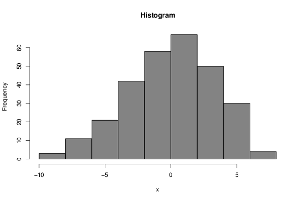
| Title produced by software | Histogram | ||||||||||||||||||||||||||||||||||||||||||||||||||||||||||||||||||||||||||||||||||||||||||||||||||||||||||||||||||||||||||||||||||||||||||||||||||||||||
| Date of computation | Wed, 10 Dec 2014 11:26:01 +0000 | ||||||||||||||||||||||||||||||||||||||||||||||||||||||||||||||||||||||||||||||||||||||||||||||||||||||||||||||||||||||||||||||||||||||||||||||||||||||||
| Cite this page as follows | Statistical Computations at FreeStatistics.org, Office for Research Development and Education, URL https://freestatistics.org/blog/index.php?v=date/2014/Dec/10/t1418210805q3sz379r8l8suog.htm/, Retrieved Sun, 19 May 2024 14:05:34 +0000 | ||||||||||||||||||||||||||||||||||||||||||||||||||||||||||||||||||||||||||||||||||||||||||||||||||||||||||||||||||||||||||||||||||||||||||||||||||||||||
| Statistical Computations at FreeStatistics.org, Office for Research Development and Education, URL https://freestatistics.org/blog/index.php?pk=264932, Retrieved Sun, 19 May 2024 14:05:34 +0000 | |||||||||||||||||||||||||||||||||||||||||||||||||||||||||||||||||||||||||||||||||||||||||||||||||||||||||||||||||||||||||||||||||||||||||||||||||||||||||
| QR Codes: | |||||||||||||||||||||||||||||||||||||||||||||||||||||||||||||||||||||||||||||||||||||||||||||||||||||||||||||||||||||||||||||||||||||||||||||||||||||||||
|
| |||||||||||||||||||||||||||||||||||||||||||||||||||||||||||||||||||||||||||||||||||||||||||||||||||||||||||||||||||||||||||||||||||||||||||||||||||||||||
| Original text written by user: | |||||||||||||||||||||||||||||||||||||||||||||||||||||||||||||||||||||||||||||||||||||||||||||||||||||||||||||||||||||||||||||||||||||||||||||||||||||||||
| IsPrivate? | No (this computation is public) | ||||||||||||||||||||||||||||||||||||||||||||||||||||||||||||||||||||||||||||||||||||||||||||||||||||||||||||||||||||||||||||||||||||||||||||||||||||||||
| User-defined keywords | |||||||||||||||||||||||||||||||||||||||||||||||||||||||||||||||||||||||||||||||||||||||||||||||||||||||||||||||||||||||||||||||||||||||||||||||||||||||||
| Estimated Impact | 88 | ||||||||||||||||||||||||||||||||||||||||||||||||||||||||||||||||||||||||||||||||||||||||||||||||||||||||||||||||||||||||||||||||||||||||||||||||||||||||
Tree of Dependent Computations | |||||||||||||||||||||||||||||||||||||||||||||||||||||||||||||||||||||||||||||||||||||||||||||||||||||||||||||||||||||||||||||||||||||||||||||||||||||||||
| Family? (F = Feedback message, R = changed R code, M = changed R Module, P = changed Parameters, D = changed Data) | |||||||||||||||||||||||||||||||||||||||||||||||||||||||||||||||||||||||||||||||||||||||||||||||||||||||||||||||||||||||||||||||||||||||||||||||||||||||||
| - [Cronbach Alpha] [Intrinsic Motivat...] [2010-10-12 11:46:14] [b98453cac15ba1066b407e146608df68] - RMPD [Cronbach Alpha] [] [2014-12-09 22:15:28] [6b382800c0d3804662889dbce999b8c7] - RMPD [Notched Boxplots] [] [2014-12-10 09:38:26] [6b382800c0d3804662889dbce999b8c7] - R D [Notched Boxplots] [] [2014-12-10 09:44:14] [6b382800c0d3804662889dbce999b8c7] - RMPD [Histogram] [] [2014-12-10 11:26:01] [6993448de96b8662e47595bfdf466bf3] [Current] | |||||||||||||||||||||||||||||||||||||||||||||||||||||||||||||||||||||||||||||||||||||||||||||||||||||||||||||||||||||||||||||||||||||||||||||||||||||||||
| Feedback Forum | |||||||||||||||||||||||||||||||||||||||||||||||||||||||||||||||||||||||||||||||||||||||||||||||||||||||||||||||||||||||||||||||||||||||||||||||||||||||||
Post a new message | |||||||||||||||||||||||||||||||||||||||||||||||||||||||||||||||||||||||||||||||||||||||||||||||||||||||||||||||||||||||||||||||||||||||||||||||||||||||||
Dataset | |||||||||||||||||||||||||||||||||||||||||||||||||||||||||||||||||||||||||||||||||||||||||||||||||||||||||||||||||||||||||||||||||||||||||||||||||||||||||
| Dataseries X: | |||||||||||||||||||||||||||||||||||||||||||||||||||||||||||||||||||||||||||||||||||||||||||||||||||||||||||||||||||||||||||||||||||||||||||||||||||||||||
-0,932343 -6,93751 -0,153995 -1,26882 -4,352 -5,16395 1,24985 -0,00577569 0,0753537 -0,87223 -4,18554 -1,30858 -5,82164 -1,75675 -1,52103 -7,14674 -1,78067 -0,805482 -3,84196 -1,70174 -2,84754 -6,08901 1,8923 -2,20805 1,52879 -2,03975 -0,842343 4,1337 -0,266316 -3,36874 -2,77459 -4,71072 -1,41622 -6,85399 -4,0306 -3,20961 -2,35945 -3,76688 -2,88869 0,694623 -3,81923 -2,35161 -7,21958 -1,82887 0,597197 -2,5172 0,142261 -3,20274 0,425312 -3,76359 0,76412 -0,38652 -1,90772 -4,82032 -2,68886 0,757643 0,777656 -3,39756 -8,23879 3,26931 -4,80957 1,14018 -4,13672 -0,193295 -7,53944 2,8151 -3,91622 -3,82707 -3,32881 -0,00829538 0,814966 -0,827151 -0,976729 -2,52133 -4,53535 2,12512 -5,70245 -0,538191 -0,220272 5,77E-05 -0,53168 -2,8334 -4,15335 -2,75487 0,926821 -2,86148 -7,40381 -2,92332 0,246003 -1,17476 -2,58725 -5,47279 1,25415 0,145427 -6,55047 -0,807706 -4,59654 -3,14515 -2,91593 -4,25982 -1,78403 1,26256 -4,66386 -1,92292 -3,99028 -2,42777 -1,59663 2,9061 -4,10674 1,22893 -8,81813 -6,82817 -2,93204 -1,89102 -0,920299 -7,96448 -1,11297 4,76162 3,40514 2,30939 1,26557 4,07216 3,90352 3,64147 0,201754 4,4769 1,75495 -2,17429 1,27342 4,69019 1,69783 6,665 0,837149 0,24104 2,69079 1,8991 1,99346 -1,42577 0,385293 3,67447 -4,61032 4,46897 2,88118 -1,62456 4,79743 3,96682 4,42113 2,46181 2,70047 3,68022 1,93659 -1,57563 0,727305 1,72528 4,17729 -3,24789 2,2606 5,44239 4,05359 1,18126 2,32385 4,91746 1,54566 1,45203 -2,52856 4,33116 3,48216 2,30281 2,16197 4,93456 -1,74403 4,81768 1,00884 0,961538 -2,54927 3,20609 4,93642 1,61455 1,81346 1,81346 5,71029 0,721124 6,5277 3,20166 -5,68328 -0,283099 0,919556 5,32037 2,63386 0,0909615 2,65191 3,90191 -0,298088 -1,24963 1,72848 -2,03625 2,92044 -3,01499 5,85464 0,957987 1,52265 1,07297 1,72582 2,13369 3,22561 6,79147 2,09446 0,267959 1,39749 -0,149357 0,612753 -2,02367 0,483979 0,20624 7,15744 4,02144 -1,89505 2,52386 -1,15913 0,696459 2,87975 1,66967 3,59513 0,725288 4,42637 -1,0606 2,11525 4,5554 -5,55071 -0,686779 3,36487 3,99497 1,80857 3,19035 2,4527 5,23231 5,00184 5,8833 4,81238 0,438872 -0,235254 -1,83164 -8,49351 -0,776198 1,38897 0,416817 0,532063 -1,07649 -0,74235 2,75464 4,93456 4,1724 -1,00035 2,67596 4,15148 1,26791 2,75968 1,07844 -0,0662818 -2,15722 1,71199 2,70773 -0,11166 3,08883 -4,75021 -6,65185 -0,280772 -2,86038 -1,74403 -1,45963 -1,45913 2,75464 2,4199 -0,217014 0,382371 3,89367 3,74675 -2,31064 2,60426 -0,956236 2,82273 4,0287 3,25808 0,446726 3,25857 -3,86352 | |||||||||||||||||||||||||||||||||||||||||||||||||||||||||||||||||||||||||||||||||||||||||||||||||||||||||||||||||||||||||||||||||||||||||||||||||||||||||
Tables (Output of Computation) | |||||||||||||||||||||||||||||||||||||||||||||||||||||||||||||||||||||||||||||||||||||||||||||||||||||||||||||||||||||||||||||||||||||||||||||||||||||||||
| |||||||||||||||||||||||||||||||||||||||||||||||||||||||||||||||||||||||||||||||||||||||||||||||||||||||||||||||||||||||||||||||||||||||||||||||||||||||||
Figures (Output of Computation) | |||||||||||||||||||||||||||||||||||||||||||||||||||||||||||||||||||||||||||||||||||||||||||||||||||||||||||||||||||||||||||||||||||||||||||||||||||||||||
Input Parameters & R Code | |||||||||||||||||||||||||||||||||||||||||||||||||||||||||||||||||||||||||||||||||||||||||||||||||||||||||||||||||||||||||||||||||||||||||||||||||||||||||
| Parameters (Session): | |||||||||||||||||||||||||||||||||||||||||||||||||||||||||||||||||||||||||||||||||||||||||||||||||||||||||||||||||||||||||||||||||||||||||||||||||||||||||
| Parameters (R input): | |||||||||||||||||||||||||||||||||||||||||||||||||||||||||||||||||||||||||||||||||||||||||||||||||||||||||||||||||||||||||||||||||||||||||||||||||||||||||
| par1 = ; par2 = grey ; par3 = FALSE ; par4 = Unknown ; | |||||||||||||||||||||||||||||||||||||||||||||||||||||||||||||||||||||||||||||||||||||||||||||||||||||||||||||||||||||||||||||||||||||||||||||||||||||||||
| R code (references can be found in the software module): | |||||||||||||||||||||||||||||||||||||||||||||||||||||||||||||||||||||||||||||||||||||||||||||||||||||||||||||||||||||||||||||||||||||||||||||||||||||||||
par1 <- as.numeric(par1) | |||||||||||||||||||||||||||||||||||||||||||||||||||||||||||||||||||||||||||||||||||||||||||||||||||||||||||||||||||||||||||||||||||||||||||||||||||||||||