Free Statistics
of Irreproducible Research!
Description of Statistical Computation | |||||||||||||||||||||
|---|---|---|---|---|---|---|---|---|---|---|---|---|---|---|---|---|---|---|---|---|---|
| Author's title | |||||||||||||||||||||
| Author | *Unverified author* | ||||||||||||||||||||
| R Software Module | rwasp_sdplot.wasp | ||||||||||||||||||||
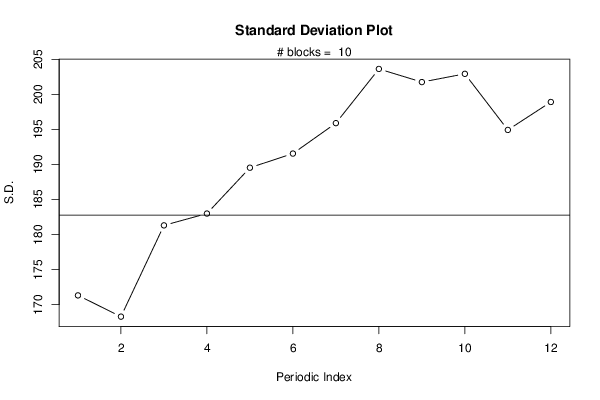
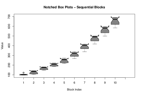
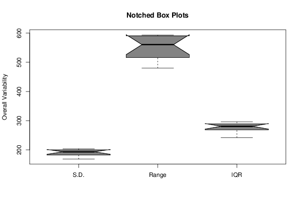
| Title produced by software | Standard Deviation Plot | ||||||||||||||||||||
| Date of computation | Wed, 13 Aug 2014 10:51:12 +0100 | ||||||||||||||||||||
| Cite this page as follows | Statistical Computations at FreeStatistics.org, Office for Research Development and Education, URL https://freestatistics.org/blog/index.php?v=date/2014/Aug/13/t1407923587fynkh4v7r8u3hay.htm/, Retrieved Wed, 15 May 2024 19:49:37 +0000 | ||||||||||||||||||||
| Statistical Computations at FreeStatistics.org, Office for Research Development and Education, URL https://freestatistics.org/blog/index.php?pk=235497, Retrieved Wed, 15 May 2024 19:49:37 +0000 | |||||||||||||||||||||
| QR Codes: | |||||||||||||||||||||
|
| |||||||||||||||||||||
| Original text written by user: | |||||||||||||||||||||
| IsPrivate? | No (this computation is public) | ||||||||||||||||||||
| User-defined keywords | |||||||||||||||||||||
| Estimated Impact | 90 | ||||||||||||||||||||
Tree of Dependent Computations | |||||||||||||||||||||
| Family? (F = Feedback message, R = changed R code, M = changed R Module, P = changed Parameters, D = changed Data) | |||||||||||||||||||||
| - [(Partial) Autocorrelation Function] [] [2014-08-13 09:41:06] [ba0170e6f15797e8c541ec0953bc1848] - RMP [Standard Deviation Plot] [] [2014-08-13 09:51:12] [b3e3d38149b35cb70244b37a39776b3a] [Current] | |||||||||||||||||||||
| Feedback Forum | |||||||||||||||||||||
Post a new message | |||||||||||||||||||||
Dataset | |||||||||||||||||||||
| Dataseries X: | |||||||||||||||||||||
106 105 104 102 122 121 106 96 97 97 98 100 106 104 107 112 140 140 134 128 133 139 140 143 152 146 146 155 180 182 177 165 174 174 175 180 184 186 186 192 215 221 222 207 215 212 206 219 222 217 218 225 251 264 264 258 267 258 253 272 275 268 286 293 314 328 326 325 333 332 320 338 344 338 363 375 403 414 411 405 410 416 396 412 422 418 444 453 491 498 489 494 497 500 481 499 509 499 528 537 576 582 584 594 594 598 580 589 595 584 616 622 662 669 679 688 689 690 672 690 | |||||||||||||||||||||
Tables (Output of Computation) | |||||||||||||||||||||
| |||||||||||||||||||||
Figures (Output of Computation) | |||||||||||||||||||||
Input Parameters & R Code | |||||||||||||||||||||
| Parameters (Session): | |||||||||||||||||||||
| par1 = Default ; par2 = 1 ; par3 = 0 ; par4 = 0 ; par5 = 12 ; par6 = White Noise ; par7 = 0.95 ; par8 = 48 ; | |||||||||||||||||||||
| Parameters (R input): | |||||||||||||||||||||
| par1 = 12 ; | |||||||||||||||||||||
| R code (references can be found in the software module): | |||||||||||||||||||||
par1 <- as.numeric(par1) | |||||||||||||||||||||