Free Statistics
of Irreproducible Research!
Description of Statistical Computation | |||||||||||||||||||||
|---|---|---|---|---|---|---|---|---|---|---|---|---|---|---|---|---|---|---|---|---|---|
| Author's title | |||||||||||||||||||||
| Author | *Unverified author* | ||||||||||||||||||||
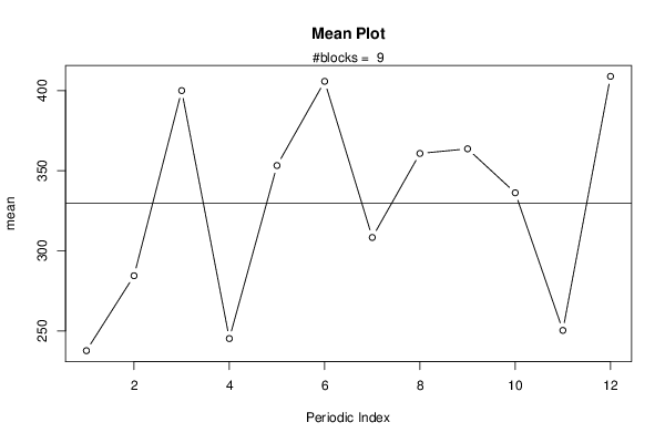
| R Software Module | rwasp_meanplot.wasp | ||||||||||||||||||||
| Title produced by software | Mean Plot | ||||||||||||||||||||
| Date of computation | Tue, 05 Aug 2014 14:23:08 +0100 | ||||||||||||||||||||
| Cite this page as follows | Statistical Computations at FreeStatistics.org, Office for Research Development and Education, URL https://freestatistics.org/blog/index.php?v=date/2014/Aug/05/t14072451638369chygvtd7wpb.htm/, Retrieved Fri, 17 May 2024 11:08:16 +0000 | ||||||||||||||||||||
| Statistical Computations at FreeStatistics.org, Office for Research Development and Education, URL https://freestatistics.org/blog/index.php?pk=235408, Retrieved Fri, 17 May 2024 11:08:16 +0000 | |||||||||||||||||||||
| QR Codes: | |||||||||||||||||||||
|
| |||||||||||||||||||||
| Original text written by user: | |||||||||||||||||||||
| IsPrivate? | No (this computation is public) | ||||||||||||||||||||
| User-defined keywords | Ines Van Dessel | ||||||||||||||||||||
| Estimated Impact | 123 | ||||||||||||||||||||
Tree of Dependent Computations | |||||||||||||||||||||
| Family? (F = Feedback message, R = changed R code, M = changed R Module, P = changed Parameters, D = changed Data) | |||||||||||||||||||||
| - [Histogram] [Tijdreeks 1 - Stap 3] [2014-08-03 19:11:32] [ae3d1feb555b13e324db089723206180] - R P [Histogram] [Tijdreeks 1 - Stap 5] [2014-08-04 09:44:37] [74be16979710d4c4e7c6647856088456] - P [Histogram] [Tijdreeks 1 - Stap 5] [2014-08-04 09:47:49] [74be16979710d4c4e7c6647856088456] - RMP [(Partial) Autocorrelation Function] [Tijdreeks 1 - Sta...] [2014-08-04 16:49:46] [ae3d1feb555b13e324db089723206180] - R P [(Partial) Autocorrelation Function] [Tijdreeks 1 - Sta...] [2014-08-05 08:15:03] [74be16979710d4c4e7c6647856088456] - RMPD [Harrell-Davis Quantiles] [Tijdreeks 2 - Stap 6] [2014-08-05 08:50:48] [ae3d1feb555b13e324db089723206180] - RMP [Mean Plot] [Tijdreeks 2 - Sta...] [2014-08-05 13:23:08] [188bf81caccb86647293be436f272d1b] [Current] | |||||||||||||||||||||
| Feedback Forum | |||||||||||||||||||||
Post a new message | |||||||||||||||||||||
Dataset | |||||||||||||||||||||
| Dataseries X: | |||||||||||||||||||||
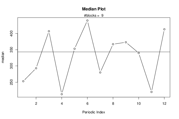
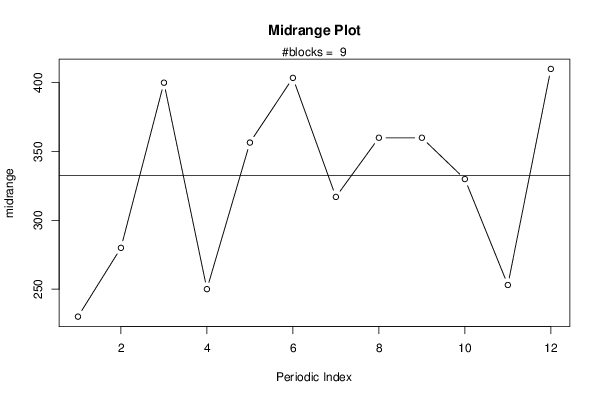
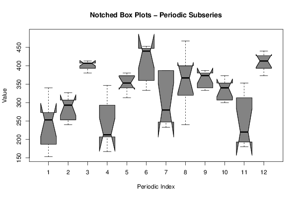
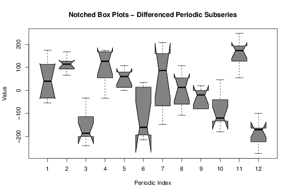
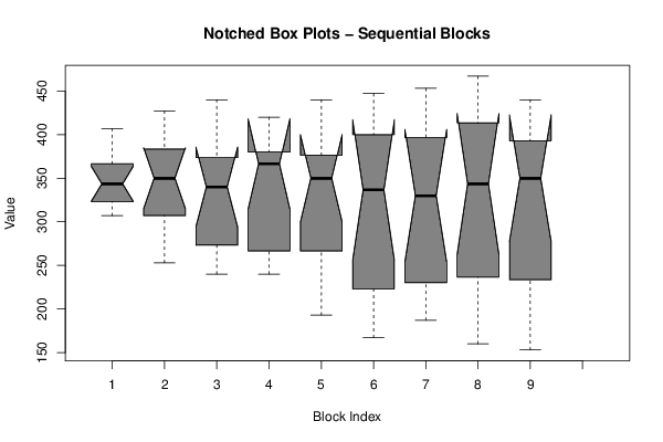
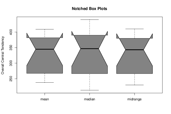
340 307 380 347 313 333 347 333 387 307 353 407 307 253 380 320 353 353 387 280 387 307 347 427 253 240 407 293 347 360 387 240 333 353 313 440 273 240 407 240 360 373 387 320 373 373 260 420 253 293 413 207 333 440 280 367 380 373 193 373 213 293 407 167 340 447 233 393 333 353 200 413 187 300 413 213 373 453 247 447 340 320 187 380 160 307 400 213 380 453 260 467 380 300 180 427 153 327 393 207 380 440 247 400 360 340 220 393 | |||||||||||||||||||||
Tables (Output of Computation) | |||||||||||||||||||||
| |||||||||||||||||||||
Figures (Output of Computation) | |||||||||||||||||||||
Input Parameters & R Code | |||||||||||||||||||||
| Parameters (Session): | |||||||||||||||||||||
| Parameters (R input): | |||||||||||||||||||||
| par1 = 12 ; | |||||||||||||||||||||
| R code (references can be found in the software module): | |||||||||||||||||||||
par1 <- as.numeric(par1) | |||||||||||||||||||||