Free Statistics
of Irreproducible Research!
Description of Statistical Computation | |||||||||||||||||||||
|---|---|---|---|---|---|---|---|---|---|---|---|---|---|---|---|---|---|---|---|---|---|
| Author's title | |||||||||||||||||||||
| Author | *Unverified author* | ||||||||||||||||||||
| R Software Module | rwasp_meanplot.wasp | ||||||||||||||||||||
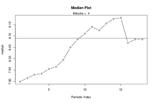
| Title produced by software | Mean Plot | ||||||||||||||||||||
| Date of computation | Tue, 23 Oct 2012 15:13:29 -0400 | ||||||||||||||||||||
| Cite this page as follows | Statistical Computations at FreeStatistics.org, Office for Research Development and Education, URL https://freestatistics.org/blog/index.php?v=date/2012/Oct/23/t1351019723lemly0w79bnbxwp.htm/, Retrieved Thu, 02 May 2024 07:13:08 +0000 | ||||||||||||||||||||
| Statistical Computations at FreeStatistics.org, Office for Research Development and Education, URL https://freestatistics.org/blog/index.php?pk=183268, Retrieved Thu, 02 May 2024 07:13:08 +0000 | |||||||||||||||||||||
| QR Codes: | |||||||||||||||||||||
|
| |||||||||||||||||||||
| Original text written by user: | |||||||||||||||||||||
| IsPrivate? | No (this computation is public) | ||||||||||||||||||||
| User-defined keywords | |||||||||||||||||||||
| Estimated Impact | 100 | ||||||||||||||||||||
Tree of Dependent Computations | |||||||||||||||||||||
| Family? (F = Feedback message, R = changed R code, M = changed R Module, P = changed Parameters, D = changed Data) | |||||||||||||||||||||
| - [Mean Plot] [Mean Plot Pizza] [2012-10-23 19:13:29] [fd7ec8291d4731160120df3dd57458b8] [Current] - R [Mean Plot] [] [2013-01-02 12:37:44] [74be16979710d4c4e7c6647856088456] | |||||||||||||||||||||
| Feedback Forum | |||||||||||||||||||||
Post a new message | |||||||||||||||||||||
Dataset | |||||||||||||||||||||
| Dataseries X: | |||||||||||||||||||||
7.66 7.53 7.54 7.56 7.57 7.56 7.57 7.61 7.61 7.6 7.61 7.61 7.62 7.7 7.73 7.75 7.76 7.76 7.77 7.79 7.79 7.79 7.83 7.83 7.88 7.95 8.01 8.05 8.1 8.1 8.16 8.18 8.2 7.99 8.01 8.02 8.03 8.04 8.07 8.08 8.08 8.1 8.11 8.15 8.16 8.17 8.18 8.15 8.15 8.17 8.16 8.15 8.16 8.15 8.18 8.19 8.18 8.2 8.21 8.22 8.23 8.25 8.28 8.28 8.29 8.3 8.34 8.38 8.39 8.44 8.46 8.46 | |||||||||||||||||||||
Tables (Output of Computation) | |||||||||||||||||||||
| |||||||||||||||||||||
Figures (Output of Computation) | |||||||||||||||||||||
Input Parameters & R Code | |||||||||||||||||||||
| Parameters (Session): | |||||||||||||||||||||
| par1 = 18 ; | |||||||||||||||||||||
| Parameters (R input): | |||||||||||||||||||||
| par1 = 18 ; | |||||||||||||||||||||
| R code (references can be found in the software module): | |||||||||||||||||||||
par1 <- '12' | |||||||||||||||||||||