Free Statistics
of Irreproducible Research!
Description of Statistical Computation | |||||||||||||||||||||
|---|---|---|---|---|---|---|---|---|---|---|---|---|---|---|---|---|---|---|---|---|---|
| Author's title | |||||||||||||||||||||
| Author | *Unverified author* | ||||||||||||||||||||
| R Software Module | rwasp_meanplot.wasp | ||||||||||||||||||||
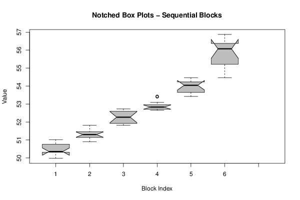
| Title produced by software | Mean Plot | ||||||||||||||||||||
| Date of computation | Sun, 21 Oct 2012 08:41:12 -0400 | ||||||||||||||||||||
| Cite this page as follows | Statistical Computations at FreeStatistics.org, Office for Research Development and Education, URL https://freestatistics.org/blog/index.php?v=date/2012/Oct/21/t1350823288wr4sm241zg2k4zk.htm/, Retrieved Mon, 29 Apr 2024 02:39:35 +0000 | ||||||||||||||||||||
| Statistical Computations at FreeStatistics.org, Office for Research Development and Education, URL https://freestatistics.org/blog/index.php?pk=180881, Retrieved Mon, 29 Apr 2024 02:39:35 +0000 | |||||||||||||||||||||
| QR Codes: | |||||||||||||||||||||
|
| |||||||||||||||||||||
| Original text written by user: | |||||||||||||||||||||
| IsPrivate? | No (this computation is public) | ||||||||||||||||||||
| User-defined keywords | |||||||||||||||||||||
| Estimated Impact | 55 | ||||||||||||||||||||
Tree of Dependent Computations | |||||||||||||||||||||
| Family? (F = Feedback message, R = changed R code, M = changed R Module, P = changed Parameters, D = changed Data) | |||||||||||||||||||||
| - [Mean Plot] [] [2012-10-21 12:41:12] [b91e71fa3b5e2ab5567c9d258a8f1839] [Current] | |||||||||||||||||||||
| Feedback Forum | |||||||||||||||||||||
Post a new message | |||||||||||||||||||||
Dataset | |||||||||||||||||||||
| Dataseries X: | |||||||||||||||||||||
49,98 50,12 50,37 50,39 50,34 50,32 50,32 50,32 50,67 50,86 50,95 51,02 51,02 51,06 50,9 51,23 51,29 51,3 51,3 51,3 51,46 51,47 51,77 51,82 51,82 51,84 51,9 51,94 52,22 52,27 52,27 52,28 52,53 52,73 52,72 52,67 52,67 52,65 52,69 52,73 52,84 52,83 52,83 52,84 52,82 53,09 53,4 53,43 53,43 53,42 53,6 53,69 54,05 54,04 54,04 54,08 54,05 54,39 54,38 54,46 54,46 54,69 54,91 55,52 56,01 56,07 56,07 56,09 56,29 56,45 56,87 56,87 | |||||||||||||||||||||
Tables (Output of Computation) | |||||||||||||||||||||
| |||||||||||||||||||||
Figures (Output of Computation) | |||||||||||||||||||||
Input Parameters & R Code | |||||||||||||||||||||
| Parameters (Session): | |||||||||||||||||||||
| par1 = 12 ; | |||||||||||||||||||||
| Parameters (R input): | |||||||||||||||||||||
| par1 = 12 ; | |||||||||||||||||||||
| R code (references can be found in the software module): | |||||||||||||||||||||
par1 <- as.numeric(par1) | |||||||||||||||||||||