Free Statistics
of Irreproducible Research!
Description of Statistical Computation | |||||||||||||||||||||
|---|---|---|---|---|---|---|---|---|---|---|---|---|---|---|---|---|---|---|---|---|---|
| Author's title | |||||||||||||||||||||
| Author | *Unverified author* | ||||||||||||||||||||
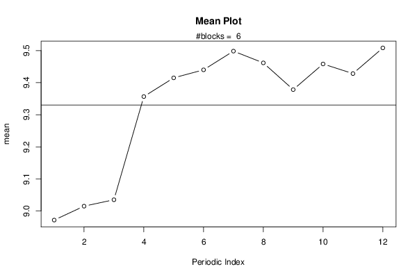
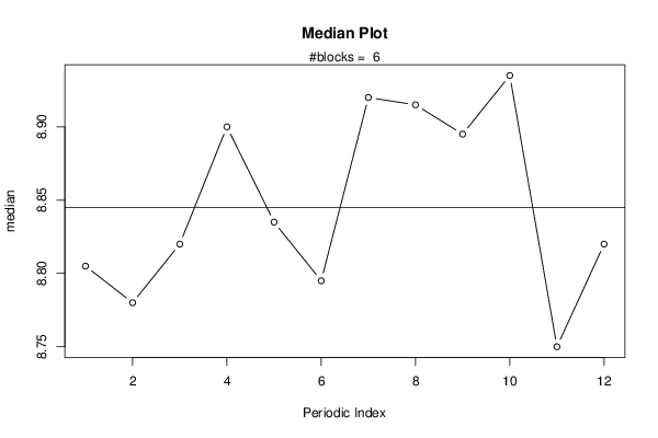
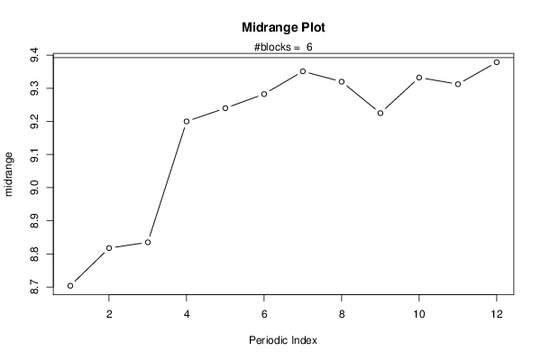
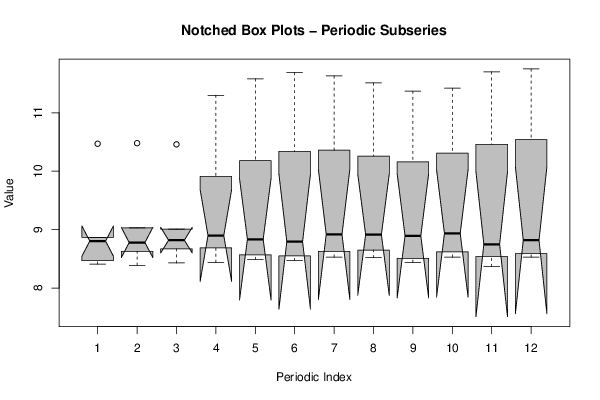
| R Software Module | rwasp_meanplot.wasp | ||||||||||||||||||||
| Title produced by software | Mean Plot | ||||||||||||||||||||
| Date of computation | Fri, 19 Oct 2012 03:38:23 -0400 | ||||||||||||||||||||
| Cite this page as follows | Statistical Computations at FreeStatistics.org, Office for Research Development and Education, URL https://freestatistics.org/blog/index.php?v=date/2012/Oct/19/t1350632458ybbe7fatxde91kc.htm/, Retrieved Mon, 29 Apr 2024 15:41:24 +0000 | ||||||||||||||||||||
| Statistical Computations at FreeStatistics.org, Office for Research Development and Education, URL https://freestatistics.org/blog/index.php?pk=179890, Retrieved Mon, 29 Apr 2024 15:41:24 +0000 | |||||||||||||||||||||
| QR Codes: | |||||||||||||||||||||
|
| |||||||||||||||||||||
| Original text written by user: | |||||||||||||||||||||
| IsPrivate? | No (this computation is public) | ||||||||||||||||||||
| User-defined keywords | |||||||||||||||||||||
| Estimated Impact | 92 | ||||||||||||||||||||
Tree of Dependent Computations | |||||||||||||||||||||
| Family? (F = Feedback message, R = changed R code, M = changed R Module, P = changed Parameters, D = changed Data) | |||||||||||||||||||||
| - [Mean Plot] [mean , medan en n...] [2012-10-19 07:38:23] [a65efd8010de7ce8a50260769e922377] [Current] | |||||||||||||||||||||
| Feedback Forum | |||||||||||||||||||||
Post a new message | |||||||||||||||||||||
Dataset | |||||||||||||||||||||
| Dataseries X: | |||||||||||||||||||||
8,41 8,39 8,43 8,44 8,49 8,47 8,53 8,52 8,51 8,53 8,54 8,53 8,47 8,63 8,67 8,73 8,57 8,55 8,63 8,65 8,44 8,62 8,37 8,59 8,84 8,72 8,8 8,69 8,68 8,57 8,85 8,85 8,85 8,93 8,75 8,78 8,77 9,03 9,01 9,07 8,99 9,02 8,99 8,98 8,94 8,94 8,75 8,86 8,87 8,84 8,84 9,91 10,18 10,34 10,36 10,26 10,16 10,31 10,46 10,54 10,47 10,48 10,46 11,3 11,58 11,69 11,63 11,51 11,37 11,42 11,7 11,75 | |||||||||||||||||||||
Tables (Output of Computation) | |||||||||||||||||||||
| |||||||||||||||||||||
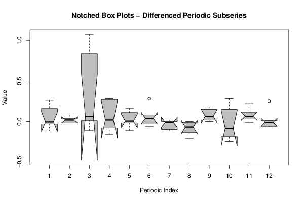
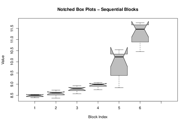
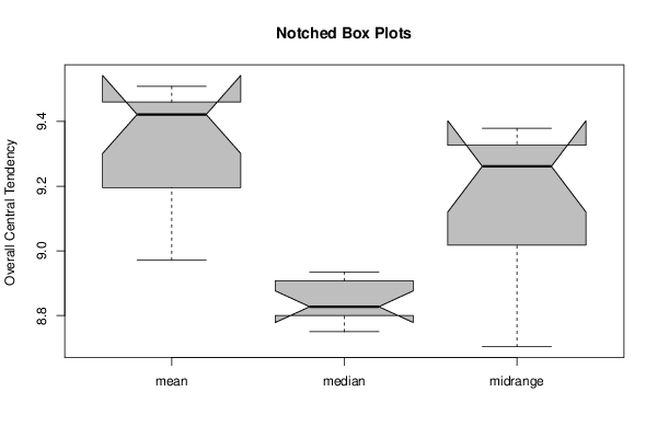
Figures (Output of Computation) | |||||||||||||||||||||
Input Parameters & R Code | |||||||||||||||||||||
| Parameters (Session): | |||||||||||||||||||||
| par1 = 12 ; | |||||||||||||||||||||
| Parameters (R input): | |||||||||||||||||||||
| par1 = 12 ; | |||||||||||||||||||||
| R code (references can be found in the software module): | |||||||||||||||||||||
par1 <- as.numeric(par1) | |||||||||||||||||||||