Free Statistics
of Irreproducible Research!
Description of Statistical Computation | |||||||||||||||||||||
|---|---|---|---|---|---|---|---|---|---|---|---|---|---|---|---|---|---|---|---|---|---|
| Author's title | |||||||||||||||||||||
| Author | *The author of this computation has been verified* | ||||||||||||||||||||
| R Software Module | rwasp_meanplot.wasp | ||||||||||||||||||||
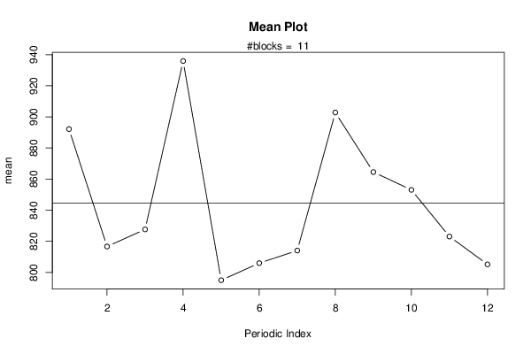
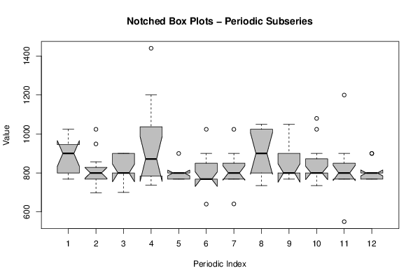
| Title produced by software | Mean Plot | ||||||||||||||||||||
| Date of computation | Tue, 02 Oct 2012 06:05:03 -0400 | ||||||||||||||||||||
| Cite this page as follows | Statistical Computations at FreeStatistics.org, Office for Research Development and Education, URL https://freestatistics.org/blog/index.php?v=date/2012/Oct/02/t1349172332ty723yqj8olv8wt.htm/, Retrieved Sat, 04 May 2024 21:17:06 +0000 | ||||||||||||||||||||
| Statistical Computations at FreeStatistics.org, Office for Research Development and Education, URL https://freestatistics.org/blog/index.php?pk=171080, Retrieved Sat, 04 May 2024 21:17:06 +0000 | |||||||||||||||||||||
| QR Codes: | |||||||||||||||||||||
|
| |||||||||||||||||||||
| Original text written by user: | |||||||||||||||||||||
| IsPrivate? | No (this computation is public) | ||||||||||||||||||||
| User-defined keywords | |||||||||||||||||||||
| Estimated Impact | 88 | ||||||||||||||||||||
Tree of Dependent Computations | |||||||||||||||||||||
| Family? (F = Feedback message, R = changed R code, M = changed R Module, P = changed Parameters, D = changed Data) | |||||||||||||||||||||
| F [Univariate Data Series] [HPC Retail Sales] [2008-03-02 15:42:48] [74be16979710d4c4e7c6647856088456] - RMPD [Mean Plot] [Weidth task 7] [2012-10-02 10:05:03] [af500d8a3ad66c35fc813daefbed0920] [Current] | |||||||||||||||||||||
| Feedback Forum | |||||||||||||||||||||
Post a new message | |||||||||||||||||||||
Dataset | |||||||||||||||||||||
| Dataseries X: | |||||||||||||||||||||
1024 768 700 768 800 1024 800 768 800 1024 800 800 1024 949 900 1200 800 800 768 735 800 845 900 768 768 768 800 1440 768 768 1024 800 900 800 900 768 900 857 800 900 800 768 768 880 768 735 1200 785 800 800 900 1050 900 768 641 1024 800 800 800 800 900 800 864 1024 800 900 800 1024 900 800 800 900 800 1024 900 768 768 800 800 900 768 800 768 800 900 800 800 880 800 900 900 1050 900 900 550 800 990 800 800 800 768 768 900 800 1024 1080 768 768 900 698 900 737 768 640 800 900 800 800 800 900 800 768 768 864 768 768 768 1050 1050 800 768 768 900 768 800 800 800 768 800 | |||||||||||||||||||||
Tables (Output of Computation) | |||||||||||||||||||||
| |||||||||||||||||||||
Figures (Output of Computation) | |||||||||||||||||||||
Input Parameters & R Code | |||||||||||||||||||||
| Parameters (Session): | |||||||||||||||||||||
| Parameters (R input): | |||||||||||||||||||||
| par1 = 12 ; | |||||||||||||||||||||
| R code (references can be found in the software module): | |||||||||||||||||||||
par1 <- as.numeric(par1) | |||||||||||||||||||||