Free Statistics

of Irreproducible Research!

Author's title

Author*Unverified author*
R Software Modulerwasp_bootstrapplot1.wasp
Title produced by softwareBootstrap Plot - Central Tendency
Date of computationFri, 30 Nov 2012 12:23:30 -0500
Cite this page as followsStatistical Computations at FreeStatistics.org, Office for Research Development and Education, URL https://freestatistics.org/blog/index.php?v=date/2012/Nov/30/t1354296247rodf55x4fh6xhuq.htm/, Retrieved Fri, 03 May 2024 19:06:47 +0000
Statistical Computations at FreeStatistics.org, Office for Research Development and Education, URL https://freestatistics.org/blog/index.php?pk=195140, Retrieved Fri, 03 May 2024 19:06:47 +0000
QR Codes:

Original text written by user:
IsPrivate?No (this computation is public)
User-defined keywords
Estimated Impact52
Family? (F = Feedback message, R = changed R code, M = changed R Module, P = changed Parameters, D = changed Data)
-       [Bootstrap Plot - Central Tendency] [] [2012-11-30 17:23:30] [de59db95ac8fc769a5d40184c39d6048] [Current]
Feedback Forum

Post a new message
Dataseries X:
20
25
15
15
25
25
25
21
30
25
20
40
13
30
25
20
25
20
25
20
20
15
15
12
20
5
20
15
25
22
20
22
25
20
20
35
30
25
20
20
20
25
25
15
20
35
25
25
30
23
10
22
25
25
22
30
20
25
25
22
25
25
25
22
25
12
18
20
20
22
30
25
22
20
50
30
25
20
30
22
25
30
22
25
22
22
25
25
25
20
22
15
20
30
20
25
30
35
22
12
30
15
10
30
9
25
20
20
35
25
35
30
12
25
15
25
25
20
20
6
15
40
20
40
25
25
20
15
15
22
24
22
20
25
25
25
35
40
20
22
22
20
25
25
18
25
20
25
30
20
22
35
22
25
25
25
25
22
23
35
15
25
18
22
25
25
28
30
20
25
25
30
22
30
10
10
25
20
22
25
25
15
22
25
25
28
22
30
25
20
25
25
20
30
20
30
50
19
20
28
20
25
35
25
25
15
16
20
20
25
30
20
25
25
25
20
20
25
25
30
22
20
25
25
18
18
20
25
25
30
25
20
25
20
20
20
22
18
22
20
15
25
25
20
25
15
22
25
25
15
12
25
30
22
15
22
25
12
18
30
25
25
40
24
25
15
25
20
25
25
25
20
30
20
25
30
22
25
25
25
50
19
50
25
35
20
20
20
20
20
25
25
25
20
20
20
20
25
18
25
22
22
30
30
8
20
25
30
50
22
20
10
25
25
25
25
18
25
20
25
30
18
20
25
22
22
20
20
25
20
20
20
20
25
20
10
20
25
30
25
50
30
30
50
15
25
25
22
20
22
30
25
18
22
22
30
40
25
20
10
20
9
15
20
15
20
30
12
15
12
20
15
12
25
20
25
25
25
30
20
25
15
15
22
10
15
10
20
25
20
20
38
20
20
20
40
25
25
30
25
10
20
25
12
15
25
20
22
22
20
25
25
25
15
40
20
20
16
25
15
20
25
20
30
50
20
25
20
30
30
25
25
12
25
25
25
20
20
20
15
20
25
15
25
50
30
20
20
25
12
15
20
20
35
22
15
18
30
22
12
12
20
20
15
25
15
20
20
25
18
30
20
25
25
25
20
20
25
20
22
15
15
22
20
10
25
20
20
15
12
20
5
20
15
15
25
25
25
15
25
22
25
20
18
22
25
35
25
25
25
35
30
22
30
50
15
25
24
20
25
25
25
12
15
22
25
25
25
25
15
20
20
15
35
30
20
22
65
20
25
22
20
25
25
20
25
15
20
12
15
10
25
15
30
35
25
25
25
25
25
40
40
25
25
20
25
25
22
25
30
25
25
30
25
25
30
25
25
20
22
22
20
25
22
25
22
40
25
25
25
22
20
35
20
35
25
22
25
25
25
25
25
40
25
30
25
20
25
25
30
22
22
20
15
15
25
25
20
20
15
25
15
20
22
25
15
15
18
5
15
25
18
40
25
25
20
30
20
25
25
25
22
22
25
25
30
25
25
25
25
20
20
25
25
25
25
20
30
25
22
30
20
20
30
25
25
30
20
25
25
24
25
30
18
15
22
22
25
22
22
25
15
20
22
18
35
20
20
20
25
25
30
15
25
22
26
25
20
25
25
25
22
25
25
20
22
30
15
30
25
20
25
25
35
22
20
25
20
20
18
20
22
25
10
20
25
20
20
30
25
20
15
20
25
10
20
25
22
22
25
25
15
25
20
10
25
16
25
35
25
15
25
25
30
25
10
22
20
25
20
20
25
22
18
30
19
25
20
25
20
25
20
22
12
30
12
22
25
25
25
25
30
30
10
22
22
25
20
22
20
25
20
15
25
20
25
20
30
15
40
25
20
22
22
30
20
40
20
25
20
25
20
50
50
25
25
40
30
22
30
20
25
25
30
25
25
20
18
18
28
25
22
15
40
40
12
12
18
12
25
26
18
25
22
15
25
15
15
15
25
15
12
22
20
20
25
20
12
9
15
12
15
25
20
20
15
15
30
21
25
22
22
50
15
25
15
25
22
18
50
20
50
20
20
30
25
20
22
25
50
40
25
25
25
25
30
40
25
30
20


Summary of computational transaction
Raw Inputview raw input (R code)
Raw Outputview raw output of R engine
Computing time14 seconds
R Server'Sir Maurice George Kendall' @ kendall.wessa.net

\begin{tabular}{lllllllll}
\hline
Summary of computational transaction \tabularnewline
Raw Input & view raw input (R code)  \tabularnewline
Raw Output & view raw output of R engine  \tabularnewline
Computing time & 14 seconds \tabularnewline
R Server & 'Sir Maurice George Kendall' @ kendall.wessa.net \tabularnewline
\hline
\end{tabular}
%Source: https://freestatistics.org/blog/index.php?pk=195140&T=0

[TABLE]
[ROW][C]Summary of computational transaction[/C][/ROW]
[ROW][C]Raw Input[/C][C]view raw input (R code) [/C][/ROW]
[ROW][C]Raw Output[/C][C]view raw output of R engine [/C][/ROW]
[ROW][C]Computing time[/C][C]14 seconds[/C][/ROW]
[ROW][C]R Server[/C][C]'Sir Maurice George Kendall' @ kendall.wessa.net[/C][/ROW]
[/TABLE]
Source: https://freestatistics.org/blog/index.php?pk=195140&T=0

Globally Unique Identifier (entire table): ba.freestatistics.org/blog/index.php?pk=195140&T=0

As an alternative you can also use a QR Code:  

The GUIDs for individual cells are displayed in the table below:

Summary of computational transaction
Raw Inputview raw input (R code)
Raw Outputview raw output of R engine
Computing time14 seconds
R Server'Sir Maurice George Kendall' @ kendall.wessa.net


Estimation Results of Bootstrap
statisticQ1EstimateQ3S.D.IQR
mean23.03323.16623.3420.226360.30972
median2222251.34433
midrange27.535353.62947.5
mode25252500
mode k.dens22.89425232.0130.10556

\begin{tabular}{lllllllll}
\hline
Estimation Results of Bootstrap \tabularnewline
statistic & Q1 & Estimate & Q3 & S.D. & IQR \tabularnewline
mean & 23.033 & 23.166 & 23.342 & 0.22636 & 0.30972 \tabularnewline
median & 22 & 22 & 25 & 1.3443 & 3 \tabularnewline
midrange & 27.5 & 35 & 35 & 3.6294 & 7.5 \tabularnewline
mode & 25 & 25 & 25 & 0 & 0 \tabularnewline
mode k.dens & 22.894 & 25 & 23 & 2.013 & 0.10556 \tabularnewline
\hline
\end{tabular}
%Source: https://freestatistics.org/blog/index.php?pk=195140&T=1

[TABLE]
[ROW][C]Estimation Results of Bootstrap[/C][/ROW]
[ROW][C]statistic[/C][C]Q1[/C][C]Estimate[/C][C]Q3[/C][C]S.D.[/C][C]IQR[/C][/ROW]
[ROW][C]mean[/C][C]23.033[/C][C]23.166[/C][C]23.342[/C][C]0.22636[/C][C]0.30972[/C][/ROW]
[ROW][C]median[/C][C]22[/C][C]22[/C][C]25[/C][C]1.3443[/C][C]3[/C][/ROW]
[ROW][C]midrange[/C][C]27.5[/C][C]35[/C][C]35[/C][C]3.6294[/C][C]7.5[/C][/ROW]
[ROW][C]mode[/C][C]25[/C][C]25[/C][C]25[/C][C]0[/C][C]0[/C][/ROW]
[ROW][C]mode k.dens[/C][C]22.894[/C][C]25[/C][C]23[/C][C]2.013[/C][C]0.10556[/C][/ROW]
[/TABLE]
Source: https://freestatistics.org/blog/index.php?pk=195140&T=1

Globally Unique Identifier (entire table): ba.freestatistics.org/blog/index.php?pk=195140&T=1

As an alternative you can also use a QR Code:  

The GUIDs for individual cells are displayed in the table below:

Estimation Results of Bootstrap
statisticQ1EstimateQ3S.D.IQR
mean23.03323.16623.3420.226360.30972
median2222251.34433
midrange27.535353.62947.5
mode25252500
mode k.dens22.89425232.0130.10556


Parameters (Session):
par1 = 200 ; par2 = 5 ; par3 = 0 ;
Parameters (R input):
par1 = 200 ; par2 = 5 ; par3 = 0 ;
R code (references can be found in the software module):
par3 <- '0'
par2 <- '5'
par1 <- '50'
par1 <- as#numeric#par1#
par2 <- as#numeric#par2#
if #par3 == '0'# bw <- NULL
if #par3 != '0'# bw <- as#numeric#par3#
if #par1 < 10# par1 = 10
if #par1 > 5000# par1 = 5000
library#modeest#
library#lattice#
library#boot#
boot#stat <- function#s,i#
{
s#mean <- mean#s#i##
s#median <- median#s#i##
s#midrange <- #max#s#i## + min#s#i### / 2
s#mode <- mlv#s#i#, method='mfv'#$M
s#kernelmode <- mlv#s#i#, method='kernel', bw=bw#$M
c#s#mean, s#median, s#midrange, s#mode, s#kernelmode#
}
bitmap#file='plot1#png'#
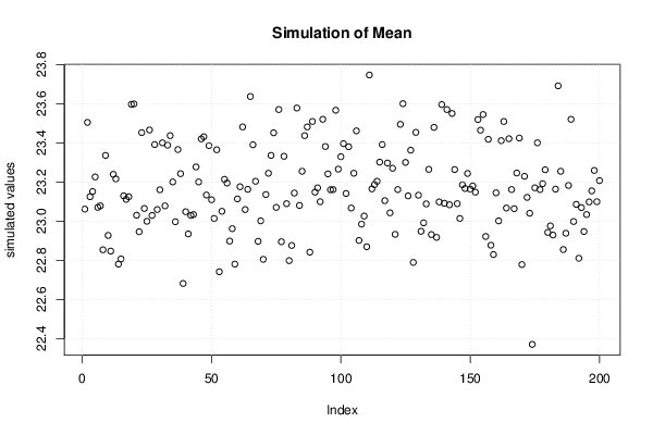
plot#r$t#,1#,type='p',ylab='simulated values',main='Simulation of Mean'#
grid##
dev#off##
bitmap#file='plot2#png'#
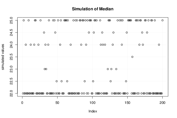
plot#r$t#,2#,type='p',ylab='simulated values',main='Simulation of Median'#
grid##
dev#off##
bitmap#file='plot3#png'#
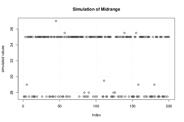
plot#r$t#,3#,type='p',ylab='simulated values',main='Simulation of Midrange'#
grid##
dev#off##
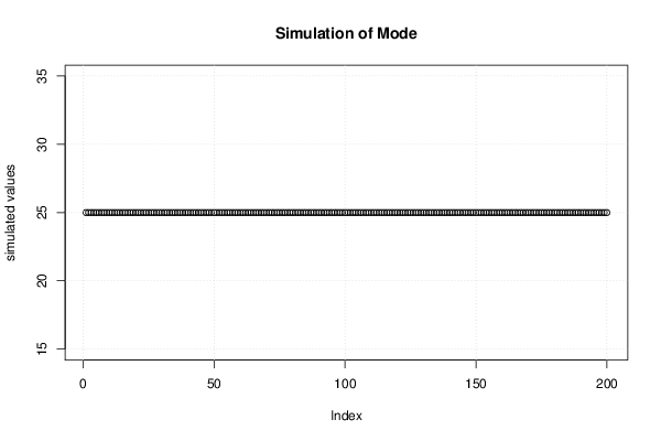
bitmap#file='plot7#png'#
plot#r$t#,4#,type='p',ylab='simulated values',main='Simulation of Mode'#
grid##
dev#off##
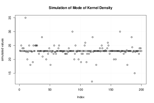
bitmap#file='plot8#png'#
plot#r$t#,5#,type='p',ylab='simulated values',main='Simulation of Mode of Kernel Density'#
grid##
dev#off##
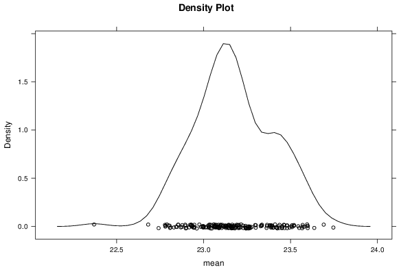
bitmap#file='plot4#png'#
densityplot#~r$t#,1#,col='black',main='Density Plot',xlab='mean'#
dev#off##
bitmap#file='plot5#png'#
densityplot#~r$t#,2#,col='black',main='Density Plot',xlab='median'#
dev#off##
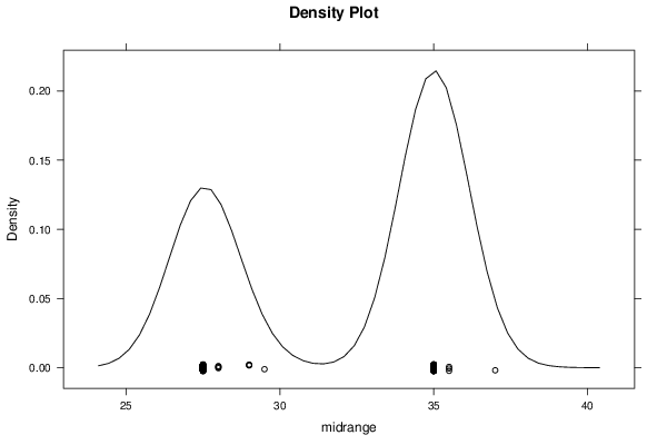
bitmap#file='plot6#png'#
densityplot#~r$t#,3#,col='black',main='Density Plot',xlab='midrange'#
dev#off##
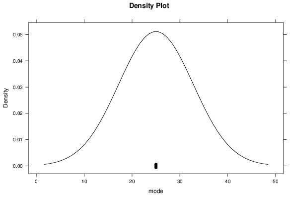
bitmap#file='plot9#png'#
densityplot#~r$t#,4#,col='black',main='Density Plot',xlab='mode'#
dev#off##
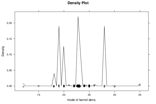
bitmap#file='plot10#png'#
densityplot#~r$t#,5#,col='black',main='Density Plot',xlab='mode of kernel dens#'#
dev#off##
z <- data#frame#cbind#r$t#,1#,r$t#,2#,r$t#,3#,r$t#,4#,r$t#,5###
colna#es#z# <- list#'mean','median','midrange','mode','mode k#dens'#
bitmap#file='plot11#png'#
boxplot#z,notch=TRUE,ylab='simulated values',main='Bootstrap Simulation - Central Tendency'#
grid##
dev#off##
load#file='createtable'#
a<-table#start##
a<-table#row#start#a#
a<-table#element#a,'Estimation Results of Bootstrap',6,TRUE#
a<-table#row#end#a#
a<-table#row#start#a#
a<-table#element#a,'statistic',header=TRUE#
a<-table#element#a,'Q1',header=TRUE#
a<-table#element#a,'Estimate',header=TRUE#
a<-table#element#a,'Q3',header=TRUE#
a<-table#element#a,'S#D#',header=TRUE#
a<-table#element#a,'IQR',header=TRUE#
a<-table#row#end#a#
a<-table#row#start#a#
a<-table#element#a,'mean',header=TRUE#
q1 <- quantile#r$t#,1#,0#25###1##
q3 <- quantile#r$t#,1#,0#75###1##
a<-table#element#a,signif#q1,par2##
a<-table#element#a,signif#r$t0#1#,par2##
a<-table#element#a,signif#q3,par2##
a<-table#element# a,signif# sqrt#var#r$t#,1###,par2 # #
a<-table#element#a,signif#q3-q1,par2##
a<-table#row#end#a#
a<-table#row#start#a#
a<-table#element#a,'median',header=TRUE#
q1 <- quantile#r$t#,2#,0#25###1##
q3 <- quantile#r$t#,2#,0#75###1##
a<-table#element#a,signif#q1,par2##
a<-table#element#a,signif#r$t0#2#,par2##
a<-table#element#a,signif#q3,par2##
a<-table#element#a,signif#sqrt#var#r$t#,2###,par2##
a<-table#element#a,signif#q3-q1,par2##
a<-table#row#end#a#
a<-table#row#start#a#
a<-table#element#a,'midrange',header=TRUE#
q1 <- quantile#r$t#,3#,0#25###1##
q3 <- quantile#r$t#,3#,0#75###1##
a<-table#element#a,signif#q1,par2##
a<-table#element#a,signif#r$t0#3#,par2##
a<-table#element#a,signif#q3,par2##
a<-table#element#a,signif#sqrt#var#r$t#,3###,par2##
a<-table#element#a,signif#q3-q1,par2##
a<-table#row#end#a#
a<-table#row#start#a#
a<-table#element#a,'mode',header=TRUE#
q1 <- quantile#r$t#,4#,0#25###1##
q3 <- quantile#r$t#,4#,0#75###1##
a<-table#element#a,signif#q1,par2##
a<-table#element#a,signif#r$t0#4#,par2##
a<-table#element#a,signif#q3,par2##
a<-table#element#a,signif#sqrt#var#r$t#,4###,par2##
a<-table#element#a,signif#q3-q1,par2##
a<-table#row#end#a#
a<-table#row#start#a#
a<-table#element#a,'mode k#dens',header=TRUE#
q1 <- quantile#r$t#,5#,0#25###1##
q3 <- quantile#r$t#,5#,0#75###1##
a<-table#element#a,signif#q1,par2##
a<-table#element#a,signif#r$t0#5#,par2##
a<-table#element#a,signif#q3,par2##
a<-table#element#a,signif#sqrt#var#r$t#,5###,par2##
a<-table#element#a,signif#q3-q1,par2##
a<-table#row#end#a#
a<-table#end#a#
table#save#a,file='mytable.tab'#