Repository of Reproducible Computations

Free Statistics

of Irreproducible Research!

Author's title

Author

*The author of this computation has been verified*

R Software Module

rwasp_autocorrelation.wasp

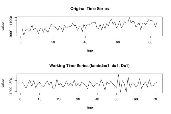
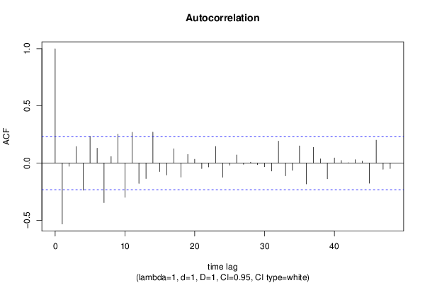
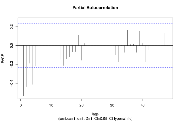
Title produced by software

(Partial) Autocorrelation Function

Date of computation

Mon, 26 Nov 2012 12:00:09 -0500

Cite this page as follows

Statistical Computations at FreeStatistics.org, Office for Research Development and Education, URL https://freestatistics.org/blog/index.php?v=date/2012/Nov/26/t1353949227rnm29aiqyzwyw5d.htm/, Retrieved Tue, 30 Apr 2024 02:32:43 +0000

Statistical Computations at FreeStatistics.org, Office for Research Development and Education, URL https://freestatistics.org/blog/index.php?pk=193339, Retrieved Tue, 30 Apr 2024 02:32:43 +0000

QR Codes:

Paste this QR Code to cite your computation.

Original text written by user:

IsPrivate?

No (this computation is public)

User-defined keywords

Estimated Impact

Family? (F = Feedback message, R = changed R code, M = changed R Module, P = changed Parameters, D = changed Data)

-     [Univariate Explorative Data Analysis] [Run Sequence gebo...] [2008-12-12 13:32:37] [76963dc1903f0f612b6153510a3818cf]
- R  D  [Univariate Explorative Data Analysis] [Run Sequence gebo...] [2008-12-17 12:14:40] [76963dc1903f0f612b6153510a3818cf]
-         [Univariate Explorative Data Analysis] [Run Sequence Plot...] [2008-12-22 18:19:51] [1ce0d16c8f4225c977b42c8fa93bc163]
- RMP       [Univariate Data Series] [Identifying Integ...] [2009-11-22 12:08:06] [b98453cac15ba1066b407e146608df68]
- RMP         [Spectral Analysis] [Births] [2010-11-29 09:38:20] [b98453cac15ba1066b407e146608df68]
- RMPD            [(Partial) Autocorrelation Function] [WS 9 ACF] [2012-11-26 17:00:09] [5bcb27a14a37b739141501b3993fea08] [Current]

Feedback Forum

Post a new message

Dataseries X:

Download CSV

Histogram

Boxplots

Summary of computational transaction
Raw Input	view raw input (R code)
Raw Output	view raw output of R engine
Computing time	5 seconds
R Server	'Herman Ole Andreas Wold' @ wold.wessa.net

\begin{tabular}{lllllllll}
\hline
Summary of computational transaction \tabularnewline
Raw Input & view raw input (R code)  \tabularnewline
Raw Output & view raw output of R engine  \tabularnewline
Computing time & 5 seconds \tabularnewline
R Server & 'Herman Ole Andreas Wold' @ wold.wessa.net \tabularnewline
\hline
\end{tabular}
%Source: https://freestatistics.org/blog/index.php?pk=193339&T=0

[TABLE]
[ROW][C]Summary of computational transaction[/C][/ROW]
[ROW][C]Raw Input[/C][C]view raw input (R code) [/C][/ROW]
[ROW][C]Raw Output[/C][C]view raw output of R engine [/C][/ROW]
[ROW][C]Computing time[/C][C]5 seconds[/C][/ROW]
[ROW][C]R Server[/C][C]'Herman Ole Andreas Wold' @ wold.wessa.net[/C][/ROW]
[/TABLE]
Source: https://freestatistics.org/blog/index.php?pk=193339&T=0

Globally Unique Identifier (entire table): ba.freestatistics.org/blog/index.php?pk=193339&T=0

As an alternative you can also use a QR Code:

The GUIDs for individual cells are displayed in the table below:

Summary of computational transaction
Raw Input	view raw input (R code)
Raw Output	view raw output of R engine
Computing time	5 seconds
R Server	'Herman Ole Andreas Wold' @ wold.wessa.net

Autocorrelation Function
Time lag k	ACF(k)	T-STAT	P-value
1	-0.533115	-4.4921	1.3e-05
2	-0.027899	-0.2351	0.407412
3	0.144781	1.2199	0.11326
4	-0.237271	-1.9993	0.024703
5	0.234261	1.9739	0.026141
6	0.130418	1.0989	0.137758
7	-0.345753	-2.9134	0.002389
8	0.056617	0.4771	0.317392
9	0.254162	2.1416	0.017829
10	-0.299487	-2.5235	0.006929
11	0.269605	2.2717	0.013068
12	-0.178019	-1.5	0.069022
13	-0.135469	-1.1415	0.128752
14	0.270791	2.2817	0.012753
15	-0.074564	-0.6283	0.265917
16	-0.103635	-0.8732	0.192736
17	0.125706	1.0592	0.146545
18	-0.122053	-1.0284	0.153617
19	0.075624	0.6372	0.263015
20	0.03341	0.2815	0.389568
21	-0.048303	-0.407	0.342614
22	-0.034375	-0.2896	0.386466
23	0.145556	1.2265	0.112035
24	-0.124158	-1.0462	0.149514
25	-0.018823	-0.1586	0.437213
26	0.071855	0.6055	0.273402
27	-0.010529	-0.0887	0.464779
28	0.007365	0.0621	0.475345
29	-0.013801	-0.1163	0.453877
30	-0.032426	-0.2732	0.392735
31	-0.069134	-0.5825	0.281025
32	0.192484	1.6219	0.054629
33	-0.111288	-0.9377	0.17578
34	-0.062642	-0.5278	0.299631
35	0.150637	1.2693	0.104241
36	-0.182658	-1.5391	0.064112
37	0.138044	1.1632	0.124326
38	0.037686	0.3176	0.375879
39	-0.137771	-1.1609	0.12479
40	0.045159	0.3805	0.35235
41	0.022815	0.1922	0.424051
42	0.003566	0.03	0.488057
43	0.029131	0.2455	0.403402
44	0.016289	0.1373	0.445608
45	-0.176347	-1.4859	0.070863
46	0.200403	1.6886	0.047839
47	-0.054068	-0.4556	0.325038
48	-0.047447	-0.3998	0.345252

\begin{tabular}{lllllllll}
\hline
Autocorrelation Function \tabularnewline
Time lag k & ACF(k) & T-STAT & P-value \tabularnewline
1 & -0.533115 & -4.4921 & 1.3e-05 \tabularnewline
2 & -0.027899 & -0.2351 & 0.407412 \tabularnewline
3 & 0.144781 & 1.2199 & 0.11326 \tabularnewline
4 & -0.237271 & -1.9993 & 0.024703 \tabularnewline
5 & 0.234261 & 1.9739 & 0.026141 \tabularnewline
6 & 0.130418 & 1.0989 & 0.137758 \tabularnewline
7 & -0.345753 & -2.9134 & 0.002389 \tabularnewline
8 & 0.056617 & 0.4771 & 0.317392 \tabularnewline
9 & 0.254162 & 2.1416 & 0.017829 \tabularnewline
10 & -0.299487 & -2.5235 & 0.006929 \tabularnewline
11 & 0.269605 & 2.2717 & 0.013068 \tabularnewline
12 & -0.178019 & -1.5 & 0.069022 \tabularnewline
13 & -0.135469 & -1.1415 & 0.128752 \tabularnewline
14 & 0.270791 & 2.2817 & 0.012753 \tabularnewline
15 & -0.074564 & -0.6283 & 0.265917 \tabularnewline
16 & -0.103635 & -0.8732 & 0.192736 \tabularnewline
17 & 0.125706 & 1.0592 & 0.146545 \tabularnewline
18 & -0.122053 & -1.0284 & 0.153617 \tabularnewline
19 & 0.075624 & 0.6372 & 0.263015 \tabularnewline
20 & 0.03341 & 0.2815 & 0.389568 \tabularnewline
21 & -0.048303 & -0.407 & 0.342614 \tabularnewline
22 & -0.034375 & -0.2896 & 0.386466 \tabularnewline
23 & 0.145556 & 1.2265 & 0.112035 \tabularnewline
24 & -0.124158 & -1.0462 & 0.149514 \tabularnewline
25 & -0.018823 & -0.1586 & 0.437213 \tabularnewline
26 & 0.071855 & 0.6055 & 0.273402 \tabularnewline
27 & -0.010529 & -0.0887 & 0.464779 \tabularnewline
28 & 0.007365 & 0.0621 & 0.475345 \tabularnewline
29 & -0.013801 & -0.1163 & 0.453877 \tabularnewline
30 & -0.032426 & -0.2732 & 0.392735 \tabularnewline
31 & -0.069134 & -0.5825 & 0.281025 \tabularnewline
32 & 0.192484 & 1.6219 & 0.054629 \tabularnewline
33 & -0.111288 & -0.9377 & 0.17578 \tabularnewline
34 & -0.062642 & -0.5278 & 0.299631 \tabularnewline
35 & 0.150637 & 1.2693 & 0.104241 \tabularnewline
36 & -0.182658 & -1.5391 & 0.064112 \tabularnewline
37 & 0.138044 & 1.1632 & 0.124326 \tabularnewline
38 & 0.037686 & 0.3176 & 0.375879 \tabularnewline
39 & -0.137771 & -1.1609 & 0.12479 \tabularnewline
40 & 0.045159 & 0.3805 & 0.35235 \tabularnewline
41 & 0.022815 & 0.1922 & 0.424051 \tabularnewline
42 & 0.003566 & 0.03 & 0.488057 \tabularnewline
43 & 0.029131 & 0.2455 & 0.403402 \tabularnewline
44 & 0.016289 & 0.1373 & 0.445608 \tabularnewline
45 & -0.176347 & -1.4859 & 0.070863 \tabularnewline
46 & 0.200403 & 1.6886 & 0.047839 \tabularnewline
47 & -0.054068 & -0.4556 & 0.325038 \tabularnewline
48 & -0.047447 & -0.3998 & 0.345252 \tabularnewline
\hline
\end{tabular}
%Source: https://freestatistics.org/blog/index.php?pk=193339&T=1

[TABLE]
[ROW][C]Autocorrelation Function[/C][/ROW]
[ROW][C]Time lag k[/C][C]ACF(k)[/C][C]T-STAT[/C][C]P-value[/C][/ROW]
[ROW][C]1[/C][C]-0.533115[/C][C]-4.4921[/C][C]1.3e-05[/C][/ROW]
[ROW][C]2[/C][C]-0.027899[/C][C]-0.2351[/C][C]0.407412[/C][/ROW]
[ROW][C]3[/C][C]0.144781[/C][C]1.2199[/C][C]0.11326[/C][/ROW]
[ROW][C]4[/C][C]-0.237271[/C][C]-1.9993[/C][C]0.024703[/C][/ROW]
[ROW][C]5[/C][C]0.234261[/C][C]1.9739[/C][C]0.026141[/C][/ROW]
[ROW][C]6[/C][C]0.130418[/C][C]1.0989[/C][C]0.137758[/C][/ROW]
[ROW][C]7[/C][C]-0.345753[/C][C]-2.9134[/C][C]0.002389[/C][/ROW]
[ROW][C]8[/C][C]0.056617[/C][C]0.4771[/C][C]0.317392[/C][/ROW]
[ROW][C]9[/C][C]0.254162[/C][C]2.1416[/C][C]0.017829[/C][/ROW]
[ROW][C]10[/C][C]-0.299487[/C][C]-2.5235[/C][C]0.006929[/C][/ROW]
[ROW][C]11[/C][C]0.269605[/C][C]2.2717[/C][C]0.013068[/C][/ROW]
[ROW][C]12[/C][C]-0.178019[/C][C]-1.5[/C][C]0.069022[/C][/ROW]
[ROW][C]13[/C][C]-0.135469[/C][C]-1.1415[/C][C]0.128752[/C][/ROW]
[ROW][C]14[/C][C]0.270791[/C][C]2.2817[/C][C]0.012753[/C][/ROW]
[ROW][C]15[/C][C]-0.074564[/C][C]-0.6283[/C][C]0.265917[/C][/ROW]
[ROW][C]16[/C][C]-0.103635[/C][C]-0.8732[/C][C]0.192736[/C][/ROW]
[ROW][C]17[/C][C]0.125706[/C][C]1.0592[/C][C]0.146545[/C][/ROW]
[ROW][C]18[/C][C]-0.122053[/C][C]-1.0284[/C][C]0.153617[/C][/ROW]
[ROW][C]19[/C][C]0.075624[/C][C]0.6372[/C][C]0.263015[/C][/ROW]
[ROW][C]20[/C][C]0.03341[/C][C]0.2815[/C][C]0.389568[/C][/ROW]
[ROW][C]21[/C][C]-0.048303[/C][C]-0.407[/C][C]0.342614[/C][/ROW]
[ROW][C]22[/C][C]-0.034375[/C][C]-0.2896[/C][C]0.386466[/C][/ROW]
[ROW][C]23[/C][C]0.145556[/C][C]1.2265[/C][C]0.112035[/C][/ROW]
[ROW][C]24[/C][C]-0.124158[/C][C]-1.0462[/C][C]0.149514[/C][/ROW]
[ROW][C]25[/C][C]-0.018823[/C][C]-0.1586[/C][C]0.437213[/C][/ROW]
[ROW][C]26[/C][C]0.071855[/C][C]0.6055[/C][C]0.273402[/C][/ROW]
[ROW][C]27[/C][C]-0.010529[/C][C]-0.0887[/C][C]0.464779[/C][/ROW]
[ROW][C]28[/C][C]0.007365[/C][C]0.0621[/C][C]0.475345[/C][/ROW]
[ROW][C]29[/C][C]-0.013801[/C][C]-0.1163[/C][C]0.453877[/C][/ROW]
[ROW][C]30[/C][C]-0.032426[/C][C]-0.2732[/C][C]0.392735[/C][/ROW]
[ROW][C]31[/C][C]-0.069134[/C][C]-0.5825[/C][C]0.281025[/C][/ROW]
[ROW][C]32[/C][C]0.192484[/C][C]1.6219[/C][C]0.054629[/C][/ROW]
[ROW][C]33[/C][C]-0.111288[/C][C]-0.9377[/C][C]0.17578[/C][/ROW]
[ROW][C]34[/C][C]-0.062642[/C][C]-0.5278[/C][C]0.299631[/C][/ROW]
[ROW][C]35[/C][C]0.150637[/C][C]1.2693[/C][C]0.104241[/C][/ROW]
[ROW][C]36[/C][C]-0.182658[/C][C]-1.5391[/C][C]0.064112[/C][/ROW]
[ROW][C]37[/C][C]0.138044[/C][C]1.1632[/C][C]0.124326[/C][/ROW]
[ROW][C]38[/C][C]0.037686[/C][C]0.3176[/C][C]0.375879[/C][/ROW]
[ROW][C]39[/C][C]-0.137771[/C][C]-1.1609[/C][C]0.12479[/C][/ROW]
[ROW][C]40[/C][C]0.045159[/C][C]0.3805[/C][C]0.35235[/C][/ROW]
[ROW][C]41[/C][C]0.022815[/C][C]0.1922[/C][C]0.424051[/C][/ROW]
[ROW][C]42[/C][C]0.003566[/C][C]0.03[/C][C]0.488057[/C][/ROW]
[ROW][C]43[/C][C]0.029131[/C][C]0.2455[/C][C]0.403402[/C][/ROW]
[ROW][C]44[/C][C]0.016289[/C][C]0.1373[/C][C]0.445608[/C][/ROW]
[ROW][C]45[/C][C]-0.176347[/C][C]-1.4859[/C][C]0.070863[/C][/ROW]
[ROW][C]46[/C][C]0.200403[/C][C]1.6886[/C][C]0.047839[/C][/ROW]
[ROW][C]47[/C][C]-0.054068[/C][C]-0.4556[/C][C]0.325038[/C][/ROW]
[ROW][C]48[/C][C]-0.047447[/C][C]-0.3998[/C][C]0.345252[/C][/ROW]
[/TABLE]
Source: https://freestatistics.org/blog/index.php?pk=193339&T=1

Globally Unique Identifier (entire table): ba.freestatistics.org/blog/index.php?pk=193339&T=1

As an alternative you can also use a QR Code:

The GUIDs for individual cells are displayed in the table below:

Autocorrelation Function
Time lag k	ACF(k)	T-STAT	P-value
1	-0.533115	-4.4921	1.3e-05
2	-0.027899	-0.2351	0.407412
3	0.144781	1.2199	0.11326
4	-0.237271	-1.9993	0.024703
5	0.234261	1.9739	0.026141
6	0.130418	1.0989	0.137758
7	-0.345753	-2.9134	0.002389
8	0.056617	0.4771	0.317392
9	0.254162	2.1416	0.017829
10	-0.299487	-2.5235	0.006929
11	0.269605	2.2717	0.013068
12	-0.178019	-1.5	0.069022
13	-0.135469	-1.1415	0.128752
14	0.270791	2.2817	0.012753
15	-0.074564	-0.6283	0.265917
16	-0.103635	-0.8732	0.192736
17	0.125706	1.0592	0.146545
18	-0.122053	-1.0284	0.153617
19	0.075624	0.6372	0.263015
20	0.03341	0.2815	0.389568
21	-0.048303	-0.407	0.342614
22	-0.034375	-0.2896	0.386466
23	0.145556	1.2265	0.112035
24	-0.124158	-1.0462	0.149514
25	-0.018823	-0.1586	0.437213
26	0.071855	0.6055	0.273402
27	-0.010529	-0.0887	0.464779
28	0.007365	0.0621	0.475345
29	-0.013801	-0.1163	0.453877
30	-0.032426	-0.2732	0.392735
31	-0.069134	-0.5825	0.281025
32	0.192484	1.6219	0.054629
33	-0.111288	-0.9377	0.17578
34	-0.062642	-0.5278	0.299631
35	0.150637	1.2693	0.104241
36	-0.182658	-1.5391	0.064112
37	0.138044	1.1632	0.124326
38	0.037686	0.3176	0.375879
39	-0.137771	-1.1609	0.12479
40	0.045159	0.3805	0.35235
41	0.022815	0.1922	0.424051
42	0.003566	0.03	0.488057
43	0.029131	0.2455	0.403402
44	0.016289	0.1373	0.445608
45	-0.176347	-1.4859	0.070863
46	0.200403	1.6886	0.047839
47	-0.054068	-0.4556	0.325038
48	-0.047447	-0.3998	0.345252

Partial Autocorrelation Function
Time lag k	PACF(k)	T-STAT	P-value
1	-0.533115	-4.4921	1.3e-05
2	-0.436037	-3.6741	0.00023
3	-0.188089	-1.5849	0.05872
4	-0.413119	-3.481	0.000429
5	-0.21966	-1.8509	0.034173
6	0.261901	2.2068	0.015281
7	0.072849	0.6138	0.270642
8	-0.262722	-2.2137	0.01503
9	0.154391	1.3009	0.098746
10	-0.044121	-0.3718	0.355585
11	-0.042324	-0.3566	0.361215
12	-0.099886	-0.8417	0.201404
13	-0.147074	-1.2393	0.109664
14	-0.211908	-1.7856	0.03922
15	-0.1423	-1.199	0.11725
16	-0.120127	-1.0122	0.157438
17	-0.067726	-0.5707	0.285012
18	-0.063938	-0.5388	0.295871
19	0.110984	0.9352	0.176436
20	-0.155848	-1.3132	0.096672
21	0.022567	0.1901	0.424867
22	0.000639	0.0054	0.49786
23	0.152246	1.2828	0.101858
24	0.08046	0.678	0.249999
25	-0.075733	-0.6381	0.262718
26	-0.178491	-1.504	0.06851
27	0.047652	0.4015	0.344621
28	-0.034066	-0.287	0.387456
29	-0.0338	-0.2848	0.388311
30	0.024193	0.2039	0.419525
31	-0.103439	-0.8716	0.193183
32	-0.174816	-1.473	0.072582
33	0.001395	0.0118	0.495329
34	-0.073022	-0.6153	0.270163
35	0.164257	1.3841	0.085339
36	0.00972	0.0819	0.467478
37	0.013779	0.1161	0.45395
38	-0.072508	-0.611	0.271587
39	0.152155	1.2821	0.101993
40	0.028141	0.2371	0.406624
41	-0.171945	-1.4488	0.075893
42	-0.043666	-0.3679	0.357009
43	-0.022225	-0.1873	0.42599
44	-0.110479	-0.9309	0.177527
45	-0.021762	-0.1834	0.427514
46	0.077523	0.6532	0.257861
47	0.130096	1.0962	0.138347
48	0.000472	0.004	0.498419

\begin{tabular}{lllllllll}
\hline
Partial Autocorrelation Function \tabularnewline
Time lag k & PACF(k) & T-STAT & P-value \tabularnewline
1 & -0.533115 & -4.4921 & 1.3e-05 \tabularnewline
2 & -0.436037 & -3.6741 & 0.00023 \tabularnewline
3 & -0.188089 & -1.5849 & 0.05872 \tabularnewline
4 & -0.413119 & -3.481 & 0.000429 \tabularnewline
5 & -0.21966 & -1.8509 & 0.034173 \tabularnewline
6 & 0.261901 & 2.2068 & 0.015281 \tabularnewline
7 & 0.072849 & 0.6138 & 0.270642 \tabularnewline
8 & -0.262722 & -2.2137 & 0.01503 \tabularnewline
9 & 0.154391 & 1.3009 & 0.098746 \tabularnewline
10 & -0.044121 & -0.3718 & 0.355585 \tabularnewline
11 & -0.042324 & -0.3566 & 0.361215 \tabularnewline
12 & -0.099886 & -0.8417 & 0.201404 \tabularnewline
13 & -0.147074 & -1.2393 & 0.109664 \tabularnewline
14 & -0.211908 & -1.7856 & 0.03922 \tabularnewline
15 & -0.1423 & -1.199 & 0.11725 \tabularnewline
16 & -0.120127 & -1.0122 & 0.157438 \tabularnewline
17 & -0.067726 & -0.5707 & 0.285012 \tabularnewline
18 & -0.063938 & -0.5388 & 0.295871 \tabularnewline
19 & 0.110984 & 0.9352 & 0.176436 \tabularnewline
20 & -0.155848 & -1.3132 & 0.096672 \tabularnewline
21 & 0.022567 & 0.1901 & 0.424867 \tabularnewline
22 & 0.000639 & 0.0054 & 0.49786 \tabularnewline
23 & 0.152246 & 1.2828 & 0.101858 \tabularnewline
24 & 0.08046 & 0.678 & 0.249999 \tabularnewline
25 & -0.075733 & -0.6381 & 0.262718 \tabularnewline
26 & -0.178491 & -1.504 & 0.06851 \tabularnewline
27 & 0.047652 & 0.4015 & 0.344621 \tabularnewline
28 & -0.034066 & -0.287 & 0.387456 \tabularnewline
29 & -0.0338 & -0.2848 & 0.388311 \tabularnewline
30 & 0.024193 & 0.2039 & 0.419525 \tabularnewline
31 & -0.103439 & -0.8716 & 0.193183 \tabularnewline
32 & -0.174816 & -1.473 & 0.072582 \tabularnewline
33 & 0.001395 & 0.0118 & 0.495329 \tabularnewline
34 & -0.073022 & -0.6153 & 0.270163 \tabularnewline
35 & 0.164257 & 1.3841 & 0.085339 \tabularnewline
36 & 0.00972 & 0.0819 & 0.467478 \tabularnewline
37 & 0.013779 & 0.1161 & 0.45395 \tabularnewline
38 & -0.072508 & -0.611 & 0.271587 \tabularnewline
39 & 0.152155 & 1.2821 & 0.101993 \tabularnewline
40 & 0.028141 & 0.2371 & 0.406624 \tabularnewline
41 & -0.171945 & -1.4488 & 0.075893 \tabularnewline
42 & -0.043666 & -0.3679 & 0.357009 \tabularnewline
43 & -0.022225 & -0.1873 & 0.42599 \tabularnewline
44 & -0.110479 & -0.9309 & 0.177527 \tabularnewline
45 & -0.021762 & -0.1834 & 0.427514 \tabularnewline
46 & 0.077523 & 0.6532 & 0.257861 \tabularnewline
47 & 0.130096 & 1.0962 & 0.138347 \tabularnewline
48 & 0.000472 & 0.004 & 0.498419 \tabularnewline
\hline
\end{tabular}
%Source: https://freestatistics.org/blog/index.php?pk=193339&T=2

[TABLE]
[ROW][C]Partial Autocorrelation Function[/C][/ROW]
[ROW][C]Time lag k[/C][C]PACF(k)[/C][C]T-STAT[/C][C]P-value[/C][/ROW]
[ROW][C]1[/C][C]-0.533115[/C][C]-4.4921[/C][C]1.3e-05[/C][/ROW]
[ROW][C]2[/C][C]-0.436037[/C][C]-3.6741[/C][C]0.00023[/C][/ROW]
[ROW][C]3[/C][C]-0.188089[/C][C]-1.5849[/C][C]0.05872[/C][/ROW]
[ROW][C]4[/C][C]-0.413119[/C][C]-3.481[/C][C]0.000429[/C][/ROW]
[ROW][C]5[/C][C]-0.21966[/C][C]-1.8509[/C][C]0.034173[/C][/ROW]
[ROW][C]6[/C][C]0.261901[/C][C]2.2068[/C][C]0.015281[/C][/ROW]
[ROW][C]7[/C][C]0.072849[/C][C]0.6138[/C][C]0.270642[/C][/ROW]
[ROW][C]8[/C][C]-0.262722[/C][C]-2.2137[/C][C]0.01503[/C][/ROW]
[ROW][C]9[/C][C]0.154391[/C][C]1.3009[/C][C]0.098746[/C][/ROW]
[ROW][C]10[/C][C]-0.044121[/C][C]-0.3718[/C][C]0.355585[/C][/ROW]
[ROW][C]11[/C][C]-0.042324[/C][C]-0.3566[/C][C]0.361215[/C][/ROW]
[ROW][C]12[/C][C]-0.099886[/C][C]-0.8417[/C][C]0.201404[/C][/ROW]
[ROW][C]13[/C][C]-0.147074[/C][C]-1.2393[/C][C]0.109664[/C][/ROW]
[ROW][C]14[/C][C]-0.211908[/C][C]-1.7856[/C][C]0.03922[/C][/ROW]
[ROW][C]15[/C][C]-0.1423[/C][C]-1.199[/C][C]0.11725[/C][/ROW]
[ROW][C]16[/C][C]-0.120127[/C][C]-1.0122[/C][C]0.157438[/C][/ROW]
[ROW][C]17[/C][C]-0.067726[/C][C]-0.5707[/C][C]0.285012[/C][/ROW]
[ROW][C]18[/C][C]-0.063938[/C][C]-0.5388[/C][C]0.295871[/C][/ROW]
[ROW][C]19[/C][C]0.110984[/C][C]0.9352[/C][C]0.176436[/C][/ROW]
[ROW][C]20[/C][C]-0.155848[/C][C]-1.3132[/C][C]0.096672[/C][/ROW]
[ROW][C]21[/C][C]0.022567[/C][C]0.1901[/C][C]0.424867[/C][/ROW]
[ROW][C]22[/C][C]0.000639[/C][C]0.0054[/C][C]0.49786[/C][/ROW]
[ROW][C]23[/C][C]0.152246[/C][C]1.2828[/C][C]0.101858[/C][/ROW]
[ROW][C]24[/C][C]0.08046[/C][C]0.678[/C][C]0.249999[/C][/ROW]
[ROW][C]25[/C][C]-0.075733[/C][C]-0.6381[/C][C]0.262718[/C][/ROW]
[ROW][C]26[/C][C]-0.178491[/C][C]-1.504[/C][C]0.06851[/C][/ROW]
[ROW][C]27[/C][C]0.047652[/C][C]0.4015[/C][C]0.344621[/C][/ROW]
[ROW][C]28[/C][C]-0.034066[/C][C]-0.287[/C][C]0.387456[/C][/ROW]
[ROW][C]29[/C][C]-0.0338[/C][C]-0.2848[/C][C]0.388311[/C][/ROW]
[ROW][C]30[/C][C]0.024193[/C][C]0.2039[/C][C]0.419525[/C][/ROW]
[ROW][C]31[/C][C]-0.103439[/C][C]-0.8716[/C][C]0.193183[/C][/ROW]
[ROW][C]32[/C][C]-0.174816[/C][C]-1.473[/C][C]0.072582[/C][/ROW]
[ROW][C]33[/C][C]0.001395[/C][C]0.0118[/C][C]0.495329[/C][/ROW]
[ROW][C]34[/C][C]-0.073022[/C][C]-0.6153[/C][C]0.270163[/C][/ROW]
[ROW][C]35[/C][C]0.164257[/C][C]1.3841[/C][C]0.085339[/C][/ROW]
[ROW][C]36[/C][C]0.00972[/C][C]0.0819[/C][C]0.467478[/C][/ROW]
[ROW][C]37[/C][C]0.013779[/C][C]0.1161[/C][C]0.45395[/C][/ROW]
[ROW][C]38[/C][C]-0.072508[/C][C]-0.611[/C][C]0.271587[/C][/ROW]
[ROW][C]39[/C][C]0.152155[/C][C]1.2821[/C][C]0.101993[/C][/ROW]
[ROW][C]40[/C][C]0.028141[/C][C]0.2371[/C][C]0.406624[/C][/ROW]
[ROW][C]41[/C][C]-0.171945[/C][C]-1.4488[/C][C]0.075893[/C][/ROW]
[ROW][C]42[/C][C]-0.043666[/C][C]-0.3679[/C][C]0.357009[/C][/ROW]
[ROW][C]43[/C][C]-0.022225[/C][C]-0.1873[/C][C]0.42599[/C][/ROW]
[ROW][C]44[/C][C]-0.110479[/C][C]-0.9309[/C][C]0.177527[/C][/ROW]
[ROW][C]45[/C][C]-0.021762[/C][C]-0.1834[/C][C]0.427514[/C][/ROW]
[ROW][C]46[/C][C]0.077523[/C][C]0.6532[/C][C]0.257861[/C][/ROW]
[ROW][C]47[/C][C]0.130096[/C][C]1.0962[/C][C]0.138347[/C][/ROW]
[ROW][C]48[/C][C]0.000472[/C][C]0.004[/C][C]0.498419[/C][/ROW]
[/TABLE]
Source: https://freestatistics.org/blog/index.php?pk=193339&T=2

Globally Unique Identifier (entire table): ba.freestatistics.org/blog/index.php?pk=193339&T=2

As an alternative you can also use a QR Code:

The GUIDs for individual cells are displayed in the table below:

Partial Autocorrelation Function
Time lag k	PACF(k)	T-STAT	P-value
1	-0.533115	-4.4921	1.3e-05
2	-0.436037	-3.6741	0.00023
3	-0.188089	-1.5849	0.05872
4	-0.413119	-3.481	0.000429
5	-0.21966	-1.8509	0.034173
6	0.261901	2.2068	0.015281
7	0.072849	0.6138	0.270642
8	-0.262722	-2.2137	0.01503
9	0.154391	1.3009	0.098746
10	-0.044121	-0.3718	0.355585
11	-0.042324	-0.3566	0.361215
12	-0.099886	-0.8417	0.201404
13	-0.147074	-1.2393	0.109664
14	-0.211908	-1.7856	0.03922
15	-0.1423	-1.199	0.11725
16	-0.120127	-1.0122	0.157438
17	-0.067726	-0.5707	0.285012
18	-0.063938	-0.5388	0.295871
19	0.110984	0.9352	0.176436
20	-0.155848	-1.3132	0.096672
21	0.022567	0.1901	0.424867
22	0.000639	0.0054	0.49786
23	0.152246	1.2828	0.101858
24	0.08046	0.678	0.249999
25	-0.075733	-0.6381	0.262718
26	-0.178491	-1.504	0.06851
27	0.047652	0.4015	0.344621
28	-0.034066	-0.287	0.387456
29	-0.0338	-0.2848	0.388311
30	0.024193	0.2039	0.419525
31	-0.103439	-0.8716	0.193183
32	-0.174816	-1.473	0.072582
33	0.001395	0.0118	0.495329
34	-0.073022	-0.6153	0.270163
35	0.164257	1.3841	0.085339
36	0.00972	0.0819	0.467478
37	0.013779	0.1161	0.45395
38	-0.072508	-0.611	0.271587
39	0.152155	1.2821	0.101993
40	0.028141	0.2371	0.406624
41	-0.171945	-1.4488	0.075893
42	-0.043666	-0.3679	0.357009
43	-0.022225	-0.1873	0.42599
44	-0.110479	-0.9309	0.177527
45	-0.021762	-0.1834	0.427514
46	0.077523	0.6532	0.257861
47	0.130096	1.0962	0.138347
48	0.000472	0.004	0.498419

Figure 1

PNG link

Postscript link

PDF link

Figure 2

PNG link

Postscript link

PDF link

Figure 3

PNG link

Postscript link

PDF link

Parameters (Session):

par1 = 48 ; par2 = 1 ; par3 = 1 ; par4 = 1 ; par5 = 12 ; par6 = White Noise ; par7 = 0.95 ;

Parameters (R input):

par1 = 48 ; par2 = 1 ; par3 = 1 ; par4 = 1 ; par5 = 12 ; par6 = White Noise ; par7 = 0.95 ; par8 = ;

R code (references can be found in the software module):

if (par1 == 'Default') {
par1 = 10*log10(length(x))
} else {
par1 <- as.numeric(par1)
}
par2 <- as.numeric(par2)
par3 <- as.numeric(par3)
par4 <- as.numeric(par4)
par5 <- as.numeric(par5)
if (par6 == 'White Noise') par6 <- 'white' else par6 <- 'ma'
par7 <- as.numeric(par7)
if (par8 != '') par8 <- as.numeric(par8)
ox <- x
if (par8 == '') {
if (par2 == 0) {
x <- log(x)
} else {
x <- (x ^ par2 - 1) / par2
}
} else {
x <- log(x,base=par8)
}
if (par3 > 0) x <- diff(x,lag=1,difference=par3)
if (par4 > 0) x <- diff(x,lag=par5,difference=par4)
bitmap(file='picts.png')
op <- par(mfrow=c(2,1))
plot(ox,type='l',main='Original Time Series',xlab='time',ylab='value')
if (par8=='') {
mytitle <- paste('Working Time Series (lambda=',par2,', d=',par3,', D=',par4,')',sep='')
mysub <- paste('(lambda=',par2,', d=',par3,', D=',par4,', CI=', par7, ', CI type=',par6,')',sep='')
} else {
mytitle <- paste('Working Time Series (base=',par8,', d=',par3,', D=',par4,')',sep='')
mysub <- paste('(base=',par8,', d=',par3,', D=',par4,', CI=', par7, ', CI type=',par6,')',sep='')
}
plot(x,type='l', main=mytitle,xlab='time',ylab='value')
par(op)
dev.off()
bitmap(file='pic1.png')
racf <- acf(x, par1, main='Autocorrelation', xlab='time lag', ylab='ACF', ci.type=par6, ci=par7, sub=mysub)
dev.off()
bitmap(file='pic2.png')
rpacf <- pacf(x,par1,main='Partial Autocorrelation',xlab='lags',ylab='PACF',sub=mysub)
dev.off()
(myacf <- c(racf$acf))
(mypacf <- c(rpacf$acf))
lengthx <- length(x)
sqrtn <- sqrt(lengthx)
load(file='createtable')
a<-table.start()
a<-table.row.start(a)
a<-table.element(a,'Autocorrelation Function',4,TRUE)
a<-table.row.end(a)
a<-table.row.start(a)
a<-table.element(a,'Time lag k',header=TRUE)
a<-table.element(a,hyperlink('basics.htm','ACF(k)','click here for more information about the Autocorrelation Function'),header=TRUE)
a<-table.element(a,'T-STAT',header=TRUE)
a<-table.element(a,'P-value',header=TRUE)
a<-table.row.end(a)
for (i in 2:(par1+1)) {
a<-table.row.start(a)
a<-table.element(a,i-1,header=TRUE)
a<-table.element(a,round(myacf[i],6))
mytstat <- myacf[i]*sqrtn
a<-table.element(a,round(mytstat,4))
a<-table.element(a,round(1-pt(abs(mytstat),lengthx),6))
a<-table.row.end(a)
}
a<-table.end(a)
table.save(a,file='mytable.tab')
a<-table.start()
a<-table.row.start(a)
a<-table.element(a,'Partial Autocorrelation Function',4,TRUE)
a<-table.row.end(a)
a<-table.row.start(a)
a<-table.element(a,'Time lag k',header=TRUE)
a<-table.element(a,hyperlink('basics.htm','PACF(k)','click here for more information about the Partial Autocorrelation Function'),header=TRUE)
a<-table.element(a,'T-STAT',header=TRUE)
a<-table.element(a,'P-value',header=TRUE)
a<-table.row.end(a)
for (i in 1:par1) {
a<-table.row.start(a)
a<-table.element(a,i,header=TRUE)
a<-table.element(a,round(mypacf[i],6))
mytstat <- mypacf[i]*sqrtn
a<-table.element(a,round(mytstat,4))
a<-table.element(a,round(1-pt(abs(mytstat),lengthx),6))
a<-table.row.end(a)
}
a<-table.end(a)
table.save(a,file='mytable1.tab')

Free Statistics

Description of Statistical Computation

Tree of Dependent Computations

Dataset

Tables (Output of Computation)

Figures (Output of Computation)

Input Parameters & R Code