Free Statistics
of Irreproducible Research!
Description of Statistical Computation | |||||||||||||||||||||
|---|---|---|---|---|---|---|---|---|---|---|---|---|---|---|---|---|---|---|---|---|---|
| Author's title | |||||||||||||||||||||
| Author | *Unverified author* | ||||||||||||||||||||
| R Software Module | rwasp_sdplot.wasp | ||||||||||||||||||||
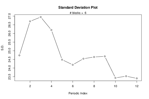
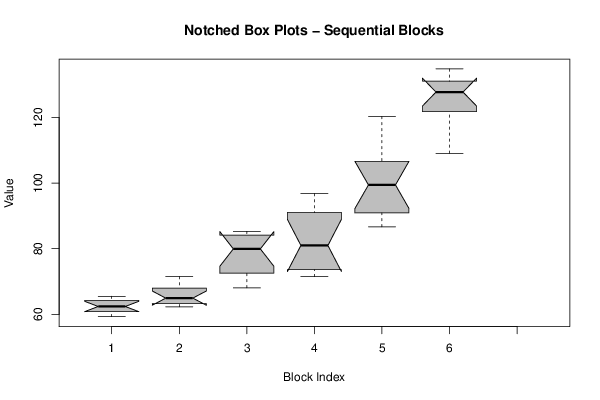
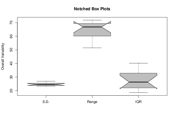
| Title produced by software | Standard Deviation Plot | ||||||||||||||||||||
| Date of computation | Mon, 26 Nov 2012 06:09:19 -0500 | ||||||||||||||||||||
| Cite this page as follows | Statistical Computations at FreeStatistics.org, Office for Research Development and Education, URL https://freestatistics.org/blog/index.php?v=date/2012/Nov/26/t13539281758y1jg1c80317ul5.htm/, Retrieved Tue, 30 Apr 2024 07:14:51 +0000 | ||||||||||||||||||||
| Statistical Computations at FreeStatistics.org, Office for Research Development and Education, URL https://freestatistics.org/blog/index.php?pk=193040, Retrieved Tue, 30 Apr 2024 07:14:51 +0000 | |||||||||||||||||||||
| QR Codes: | |||||||||||||||||||||
|
| |||||||||||||||||||||
| Original text written by user: | |||||||||||||||||||||
| IsPrivate? | No (this computation is public) | ||||||||||||||||||||
| User-defined keywords | |||||||||||||||||||||
| Estimated Impact | 69 | ||||||||||||||||||||
Tree of Dependent Computations | |||||||||||||||||||||
| Family? (F = Feedback message, R = changed R code, M = changed R Module, P = changed Parameters, D = changed Data) | |||||||||||||||||||||
| - [Standard Deviation Plot] [suiker] [2012-11-26 11:09:19] [947a57da244ad2f0e7543615f7f5630b] [Current] | |||||||||||||||||||||
| Feedback Forum | |||||||||||||||||||||
Post a new message | |||||||||||||||||||||
Dataset | |||||||||||||||||||||
| Dataseries X: | |||||||||||||||||||||
65 65,3 62,9 63,5 62,1 59,3 61,6 61,5 60,1 59,5 62,7 65,5 63,8 63,8 62,7 62,3 62,4 64,8 66,4 65,1 67,4 68,8 68,6 71,5 75 84,3 84 79,1 78,8 82,7 85,3 84,5 80,8 70,1 68,2 68,1 72,3 73,1 71,5 74,1 80,3 80,6 81,4 87,4 89,3 93,2 92,8 96,8 100,3 95,6 89 87,4 86,7 92,8 98,6 100,8 105,5 107,8 113,7 120,3 126,5 134,8 134,5 133,1 128,8 127,1 129,1 128,4 126,5 117,1 114,2 109,1 | |||||||||||||||||||||
Tables (Output of Computation) | |||||||||||||||||||||
| |||||||||||||||||||||
Figures (Output of Computation) | |||||||||||||||||||||
Input Parameters & R Code | |||||||||||||||||||||
| Parameters (Session): | |||||||||||||||||||||
| par1 = 12 ; | |||||||||||||||||||||
| Parameters (R input): | |||||||||||||||||||||
| par1 = 12 ; | |||||||||||||||||||||
| R code (references can be found in the software module): | |||||||||||||||||||||
par1 <- as.numeric(par1) | |||||||||||||||||||||