Repository of Reproducible Computations

Free Statistics

of Irreproducible Research!

Author's title

Author

*Unverified author*

R Software Module

rwasp_factor_analysis.wasp

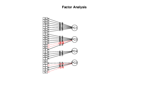
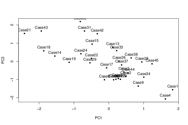
Title produced by software

Factor Analysis

Date of computation

Fri, 09 Nov 2012 11:30:44 -0500

Cite this page as follows

Statistical Computations at FreeStatistics.org, Office for Research Development and Education, URL https://freestatistics.org/blog/index.php?v=date/2012/Nov/09/t1352478773efnrpl0yb1507yr.htm/, Retrieved Mon, 29 Apr 2024 08:41:43 +0000

Statistical Computations at FreeStatistics.org, Office for Research Development and Education, URL https://freestatistics.org/blog/index.php?pk=187187, Retrieved Mon, 29 Apr 2024 08:41:43 +0000

QR Codes:

Paste this QR Code to cite your computation.

Original text written by user:

IsPrivate?

No (this computation is public)

User-defined keywords

Estimated Impact

Family? (F = Feedback message, R = changed R code, M = changed R Module, P = changed Parameters, D = changed Data)

-       [Factor Analysis] [] [2012-11-09 16:30:44] [d41d8cd98f00b204e9800998ecf8427e] [Current]

Feedback Forum

Post a new message

Dataseries X:

Download CSV

Histogram

Boxplots

'Case1'	2	2	2	4	2	5	4	5	2	2	4	5	0	0	0	0	0	1	1	0	1	0	1	1	0
'Case2'	2	2	2	2	1	4	2	5	2	2	4	2	0	1	1	1	1	0	0	0	1	1	1	1	0
'Case3'	2	2	2	5	2	2	2	2	2	2	5	5	1	1	1	0	1	1	1	1	1	1	1	1	1
'Case4'	1	1	1	4	1	4	4	4	2	2	4	4	0	0	1	1	1	1	1	1	1	0	1	1	0
'Case5'	1	1	1	2	1	2	2	2	2	2	4	4	0	1	0	0	0	0	0	0	1	0	0	1	0
'Case6'	1	1	1	2	2	4	2	2	1	1	2	4	0	1	1	1	0	1	0	0	0	1	1	1	1
'Case7'	3	4	2	NA	2	4	NA	4	4	4	4	NA	NA	NA	NA	0	1	1	0	0	1	1	NA	1	NA
'Case8'	2	2	2	2	NA	4	4	4	NA	2	4	NA	NA	0	0	1	0	1	1	0	1	1	0	1	1
'Case9'	1	2	1	2	1	2	2	4	2	4	4	4	0	0	1	0	0	1	1	0	1	0	1	1	0
'Case10'	4	2	2	2	2	2	2	2	4	NA	2	4	0	0	0	0	1	1	0	0	0	0	0	1	0
'Case12'	1	1	1	4	1	2	2	1	1	1	4	5	0	0	1	0	1	1	0	NA	0	0	1	0	0
'Case13'	2	4	4	5	2	4	4	2	4	2	4	4	0	0	0	0	1	1	1	1	0	1	0	0	0
'Case14'	2	1	1	1	1	2	1	1	1	1	2	2	0	0	1	0	1	1	0	0	0	0	0	1	0
'Case15'	4	2	2	2	2	4	2	2	4	4	4	4	0	0	1	0	1	1	0	0	0	0	0	1	0
'Case16'	2	2	4	2	2	4	NA	4	4	4	4	NA	1	1	1	0	1	1	1	0	1	0	0	1	0
'Case17'	2	2	2	2	2	2	2	2	2	4	4	4	0	0	1	0	1	1	0	0	0	0	1	0	0
'Case18'	2	2	1	2	1	1	2	1	1	1	2	1	1	0	1	0	1	1	0	0	1	0	1	0	1
'Case19'	1	1	1	1	1	2	2	2	2	2	2	2	1	1	1	0	0	1	1	1	1	0	1	1	1
'Case20'	1	2	2	2	1	2	2	4	2	2	4	4	1	0	1	1	0	0	0	0	1	0	0	1	0
'Case21'	2	4	1	1	1	2	1	1	1	1	2	2	1	1	1	1	1	1	1	1	1	0	0	1	1
'Case22'	2	2	4	2	2	2	2	2	2	2	4	4	0	1	1	0	1	0	0	1	0	0	0	1	0
'Case23'	2	2	2	4	2	4	NA	2	2	4	4	4	1	1	1	0	1	0	0	0	0	1	1	1	0
'Case24'	2	2	2	2	2	4	2	2	2	2	4	2	1	1	1	1	1	1	1	0	0	0	1	1	1
'Case25'	2	2	1	2	2	4	2	1	1	2	4	4	0	0	1	0	0	0	0	0	0	0	0	1	0
'Case26'	2	2	2	4	4	4	4	2	2	2	4	4	1	0	1	0	1	1	0	0	0	1	0	1	0
'Case27'	2	2	2	4	4	4	4	2	2	2	4	4	1	0	1	0	1	1	0	0	0	0	NA	1	0
'Case28'	4	2	2	5	2	5	4	4	4	5	4	4	0	0	1	0	1	1	0	0	0	0	1	1	0
'Case29'	2	2	2	2	2	2	2	2	2	2	2	4	0	0	0	0	1	0	0	0	0	1	1	1	0
'Case30'	2	2	1	2	1	2	2	2	4	2	4	4	0	0	1	0	1	0	1	0	1	0	1	0	0
'Case31'	4	5	2	4	2	4	2	4	4	2	4	4	1	1	1	0	1	1	0	0	0	1	0	1	0
'Case32'	4	4	4	4	2	4	2	4	4	4	4	2	0	0	0	0	1	1	0	0	0	1	0	1	0
'Case33'	4	2	2	2	2	4	4	4	4	4	5	4	0	0	0	0	0	1	0	0	1	0	0	0	1
'Case34'	2	2	2	3	2	4	2	4	3	3	4	5	0	0	1	0	1	1	0	1	1	1	1	1	0
'Case35'	2	NA	2	NA	2	4	4	4	2	4	5	4	1	1	1	0	1	0	1	0	1	0	0	1	0
'Case36'	4	2	4	NA	4	2	5	4	4	4	5	4	0	1	1	0	1	1	NA	0	1	0	0	1	0
'Case37'	1	4	2	4	2	4	5	2	2	2	4	4	0	0	1	0	1	1	0	1	0	0	0	1	0
'Case38'	4	2	4	2	2	4	2	5	4	4	5	5	0	0	1	0	1	1	0	0	0	0	1	1	0
'Case39'	1	1	1	1	1	4	1	4	1	1	4	4	0	1	NA	NA	NA	NA	NA	NA	NA	NA	NA	NA	NA
'Case40'	2	2	4	NA	5	NA	4	5	2	2	4	4	0	0	1	0	1	1	0	0	0	NA	NA	1	0
'Case41'	2	4	2	2	NA	2	2	4	4	4	4	4	0	NA	0	0	1	1	0	0	0	NA	0	1	0
'Case42'	2	4	4	2	4	4	4	2	4	4	4	4	0	0	0	0	1	1	0	0	1	0	0	1	0
'Case43'	4	4	2	2	2	2	2	2	2	2	2	2	1	1	1	1	0	1	1	1	1	0	1	1	1
'Case44'	2	2	4	2	2	4	2	4	2	2	4	2	0	0	1	1	0	1	1	0	1	1	1	0	0
'Case45'	4	4	2	4	1	5	4	5	2	4	5	5	0	0	1	0	1	1	0	0	1	1	0	1	0

Summary of computational transaction
Raw Input	view raw input (R code)
Raw Output	view raw output of R engine
Computing time	4 seconds
R Server	'Gertrude Mary Cox' @ cox.wessa.net

\begin{tabular}{lllllllll}
\hline
Summary of computational transaction \tabularnewline
Raw Input & view raw input (R code)  \tabularnewline
Raw Output & view raw output of R engine  \tabularnewline
Computing time & 4 seconds \tabularnewline
R Server & 'Gertrude Mary Cox' @ cox.wessa.net \tabularnewline
\hline
\end{tabular}
%Source: https://freestatistics.org/blog/index.php?pk=187187&T=0

[TABLE]
[ROW][C]Summary of computational transaction[/C][/ROW]
[ROW][C]Raw Input[/C][C]view raw input (R code) [/C][/ROW]
[ROW][C]Raw Output[/C][C]view raw output of R engine [/C][/ROW]
[ROW][C]Computing time[/C][C]4 seconds[/C][/ROW]
[ROW][C]R Server[/C][C]'Gertrude Mary Cox' @ cox.wessa.net[/C][/ROW]
[/TABLE]
Source: https://freestatistics.org/blog/index.php?pk=187187&T=0

Globally Unique Identifier (entire table): ba.freestatistics.org/blog/index.php?pk=187187&T=0

As an alternative you can also use a QR Code:

The GUIDs for individual cells are displayed in the table below:

Summary of computational transaction
Raw Input	view raw input (R code)
Raw Output	view raw output of R engine
Computing time	4 seconds
R Server	'Gertrude Mary Cox' @ cox.wessa.net

Rotated Factor Loadings
Variables	Factor1	Factor2	Factor3	Factor4
1a	0.088	0.754	-0.048	-0.093
1b	0.118	0.667	0.302	-0.136
1c	0.361	0.585	-0.02	-0.1
1d	0.748	-0.006	0.182	-0.389
1e	0.386	0.368	0.076	-0.393
1f	0.702	0.162	-0.025	0.066
1g	0.707	0.22	-0.008	-0.056
1h	0.595	0.273	-0.251	0.454
1i	0.25	0.775	-0.254	-0.024
1j	0.395	0.577	-0.346	0.035
1k	0.755	0.119	-0.274	0.073
1l	0.601	-0.13	-0.413	-0.226
2	-0.088	-0.021	0.725	0.046
3	-0.129	-0.048	0.528	0.214
4a	0.089	-0.432	0.362	-0.125
6	-0.139	-0.186	0.393	0.542
7	0.162	0.202	0.125	-0.655
8	0.125	0.326	0.271	-0.031
9	0.087	-0.121	0.428	0.601
10	0.017	-0.201	0.571	-0.018
11	0.068	-0.015	0.107	0.784
12	0.321	0.083	0.204	-0.036
13	0.046	-0.53	0.09	0.189
14	0.152	0.126	0.209	-0.03
15	-0.356	-0.029	0.585	0.394

\begin{tabular}{lllllllll}
\hline
Rotated Factor Loadings \tabularnewline
Variables & Factor1 & Factor2 & Factor3 & Factor4 \tabularnewline
1a & 0.088 & 0.754 & -0.048 & -0.093 \tabularnewline
1b & 0.118 & 0.667 & 0.302 & -0.136 \tabularnewline
1c & 0.361 & 0.585 & -0.02 & -0.1 \tabularnewline
1d & 0.748 & -0.006 & 0.182 & -0.389 \tabularnewline
1e & 0.386 & 0.368 & 0.076 & -0.393 \tabularnewline
1f & 0.702 & 0.162 & -0.025 & 0.066 \tabularnewline
1g & 0.707 & 0.22 & -0.008 & -0.056 \tabularnewline
1h & 0.595 & 0.273 & -0.251 & 0.454 \tabularnewline
1i & 0.25 & 0.775 & -0.254 & -0.024 \tabularnewline
1j & 0.395 & 0.577 & -0.346 & 0.035 \tabularnewline
1k & 0.755 & 0.119 & -0.274 & 0.073 \tabularnewline
1l & 0.601 & -0.13 & -0.413 & -0.226 \tabularnewline
2 & -0.088 & -0.021 & 0.725 & 0.046 \tabularnewline
3 & -0.129 & -0.048 & 0.528 & 0.214 \tabularnewline
4a & 0.089 & -0.432 & 0.362 & -0.125 \tabularnewline
6 & -0.139 & -0.186 & 0.393 & 0.542 \tabularnewline
7 & 0.162 & 0.202 & 0.125 & -0.655 \tabularnewline
8 & 0.125 & 0.326 & 0.271 & -0.031 \tabularnewline
9 & 0.087 & -0.121 & 0.428 & 0.601 \tabularnewline
10 & 0.017 & -0.201 & 0.571 & -0.018 \tabularnewline
11 & 0.068 & -0.015 & 0.107 & 0.784 \tabularnewline
12 & 0.321 & 0.083 & 0.204 & -0.036 \tabularnewline
13 & 0.046 & -0.53 & 0.09 & 0.189 \tabularnewline
14 & 0.152 & 0.126 & 0.209 & -0.03 \tabularnewline
15 & -0.356 & -0.029 & 0.585 & 0.394 \tabularnewline
\hline
\end{tabular}
%Source: https://freestatistics.org/blog/index.php?pk=187187&T=1

[TABLE]
[ROW][C]Rotated Factor Loadings[/C][/ROW]
[ROW][C]Variables[/C][C]Factor1[/C][C]Factor2[/C][C]Factor3[/C][C]Factor4[/C][/ROW]
[ROW][C]1a[/C][C]0.088[/C][C]0.754[/C][C]-0.048[/C][C]-0.093[/C][/ROW]
[ROW][C]1b[/C][C]0.118[/C][C]0.667[/C][C]0.302[/C][C]-0.136[/C][/ROW]
[ROW][C]1c[/C][C]0.361[/C][C]0.585[/C][C]-0.02[/C][C]-0.1[/C][/ROW]
[ROW][C]1d[/C][C]0.748[/C][C]-0.006[/C][C]0.182[/C][C]-0.389[/C][/ROW]
[ROW][C]1e[/C][C]0.386[/C][C]0.368[/C][C]0.076[/C][C]-0.393[/C][/ROW]
[ROW][C]1f[/C][C]0.702[/C][C]0.162[/C][C]-0.025[/C][C]0.066[/C][/ROW]
[ROW][C]1g[/C][C]0.707[/C][C]0.22[/C][C]-0.008[/C][C]-0.056[/C][/ROW]
[ROW][C]1h[/C][C]0.595[/C][C]0.273[/C][C]-0.251[/C][C]0.454[/C][/ROW]
[ROW][C]1i[/C][C]0.25[/C][C]0.775[/C][C]-0.254[/C][C]-0.024[/C][/ROW]
[ROW][C]1j[/C][C]0.395[/C][C]0.577[/C][C]-0.346[/C][C]0.035[/C][/ROW]
[ROW][C]1k[/C][C]0.755[/C][C]0.119[/C][C]-0.274[/C][C]0.073[/C][/ROW]
[ROW][C]1l[/C][C]0.601[/C][C]-0.13[/C][C]-0.413[/C][C]-0.226[/C][/ROW]
[ROW][C]2[/C][C]-0.088[/C][C]-0.021[/C][C]0.725[/C][C]0.046[/C][/ROW]
[ROW][C]3[/C][C]-0.129[/C][C]-0.048[/C][C]0.528[/C][C]0.214[/C][/ROW]
[ROW][C]4a[/C][C]0.089[/C][C]-0.432[/C][C]0.362[/C][C]-0.125[/C][/ROW]
[ROW][C]6[/C][C]-0.139[/C][C]-0.186[/C][C]0.393[/C][C]0.542[/C][/ROW]
[ROW][C]7[/C][C]0.162[/C][C]0.202[/C][C]0.125[/C][C]-0.655[/C][/ROW]
[ROW][C]8[/C][C]0.125[/C][C]0.326[/C][C]0.271[/C][C]-0.031[/C][/ROW]
[ROW][C]9[/C][C]0.087[/C][C]-0.121[/C][C]0.428[/C][C]0.601[/C][/ROW]
[ROW][C]10[/C][C]0.017[/C][C]-0.201[/C][C]0.571[/C][C]-0.018[/C][/ROW]
[ROW][C]11[/C][C]0.068[/C][C]-0.015[/C][C]0.107[/C][C]0.784[/C][/ROW]
[ROW][C]12[/C][C]0.321[/C][C]0.083[/C][C]0.204[/C][C]-0.036[/C][/ROW]
[ROW][C]13[/C][C]0.046[/C][C]-0.53[/C][C]0.09[/C][C]0.189[/C][/ROW]
[ROW][C]14[/C][C]0.152[/C][C]0.126[/C][C]0.209[/C][C]-0.03[/C][/ROW]
[ROW][C]15[/C][C]-0.356[/C][C]-0.029[/C][C]0.585[/C][C]0.394[/C][/ROW]
[/TABLE]
Source: https://freestatistics.org/blog/index.php?pk=187187&T=1

Globally Unique Identifier (entire table): ba.freestatistics.org/blog/index.php?pk=187187&T=1

As an alternative you can also use a QR Code:

The GUIDs for individual cells are displayed in the table below:

Rotated Factor Loadings
Variables	Factor1	Factor2	Factor3	Factor4
1a	0.088	0.754	-0.048	-0.093
1b	0.118	0.667	0.302	-0.136
1c	0.361	0.585	-0.02	-0.1
1d	0.748	-0.006	0.182	-0.389
1e	0.386	0.368	0.076	-0.393
1f	0.702	0.162	-0.025	0.066
1g	0.707	0.22	-0.008	-0.056
1h	0.595	0.273	-0.251	0.454
1i	0.25	0.775	-0.254	-0.024
1j	0.395	0.577	-0.346	0.035
1k	0.755	0.119	-0.274	0.073
1l	0.601	-0.13	-0.413	-0.226
2	-0.088	-0.021	0.725	0.046
3	-0.129	-0.048	0.528	0.214
4a	0.089	-0.432	0.362	-0.125
6	-0.139	-0.186	0.393	0.542
7	0.162	0.202	0.125	-0.655
8	0.125	0.326	0.271	-0.031
9	0.087	-0.121	0.428	0.601
10	0.017	-0.201	0.571	-0.018
11	0.068	-0.015	0.107	0.784
12	0.321	0.083	0.204	-0.036
13	0.046	-0.53	0.09	0.189
14	0.152	0.126	0.209	-0.03
15	-0.356	-0.029	0.585	0.394

Figure 1

PNG link

Postscript link

PDF link

Figure 2

PNG link

Postscript link

PDF link

Parameters (Session):

par1 = 4 ;

Parameters (R input):

par1 = 4 ;

R code (references can be found in the software module):

par1 <- '4'
library(psych)
par1 <- as.numeric(par1)
x <- t(x)
nrows <- length(x[,1])
ncols <- length(x[1,])
y <- array(as.double(x[1:nrows,2:ncols]),dim=c(nrows,ncols-1))
colnames(y) <- colnames(x)[2:ncols]
rownames(y) <- x[,1]
y
fit <- principal(y, nfactors=par1, rotate='varimax')
fit
fs <- factor.scores(y,fit)
fs
bitmap(file='test1.png')
fa.diagram(fit)
dev.off()
bitmap(file='test2.png')
plot(fs$scores,pch=20)
text(fs$scores,labels=rownames(y),pos=3)
dev.off()
load(file='createtable')
a<-table.start()
a<-table.row.start(a)
a<-table.element(a,'Rotated Factor Loadings',par1+1,TRUE)
a<-table.row.end(a)
a<-table.row.start(a)
a<-table.element(a,'Variables',1,TRUE)
for (i in 1:par1) {
a<-table.element(a,paste('Factor',i,sep=''),1,TRUE)
}
a<-table.row.end(a)
for (j in 1:length(fit$loadings[,1])) {
a<-table.row.start(a)
a<-table.element(a,rownames(fit$loadings)[j],header=TRUE)
for (i in 1:par1) {
a<-table.element(a,round(fit$loadings[j,i],3))
}
a<-table.row.end(a)
}
a<-table.end(a)
table.save(a,file='mytable.tab')

Free Statistics

Description of Statistical Computation

Tree of Dependent Computations

Dataset

Tables (Output of Computation)

Figures (Output of Computation)

Input Parameters & R Code