Free Statistics
of Irreproducible Research!
Description of Statistical Computation | |||||||||||||||||||||||||||||||||||||||||||||||||||||||||||||||||||||||||||||||||
|---|---|---|---|---|---|---|---|---|---|---|---|---|---|---|---|---|---|---|---|---|---|---|---|---|---|---|---|---|---|---|---|---|---|---|---|---|---|---|---|---|---|---|---|---|---|---|---|---|---|---|---|---|---|---|---|---|---|---|---|---|---|---|---|---|---|---|---|---|---|---|---|---|---|---|---|---|---|---|---|---|---|
| Author's title | |||||||||||||||||||||||||||||||||||||||||||||||||||||||||||||||||||||||||||||||||
| Author | *Unverified author* | ||||||||||||||||||||||||||||||||||||||||||||||||||||||||||||||||||||||||||||||||
| R Software Module | rwasp_bootstrapplot.wasp | ||||||||||||||||||||||||||||||||||||||||||||||||||||||||||||||||||||||||||||||||
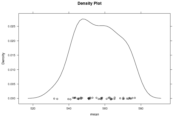
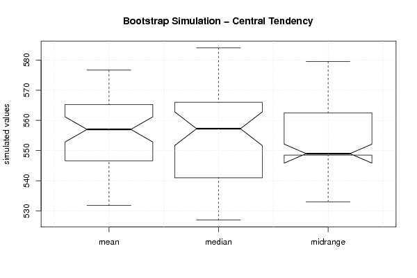
| Title produced by software | Blocked Bootstrap Plot - Central Tendency | ||||||||||||||||||||||||||||||||||||||||||||||||||||||||||||||||||||||||||||||||
| Date of computation | Fri, 25 May 2012 04:58:17 -0400 | ||||||||||||||||||||||||||||||||||||||||||||||||||||||||||||||||||||||||||||||||
| Cite this page as follows | Statistical Computations at FreeStatistics.org, Office for Research Development and Education, URL https://freestatistics.org/blog/index.php?v=date/2012/May/25/t1337936323ikkdb0njr2u85b5.htm/, Retrieved Sat, 04 May 2024 00:31:05 +0000 | ||||||||||||||||||||||||||||||||||||||||||||||||||||||||||||||||||||||||||||||||
| Statistical Computations at FreeStatistics.org, Office for Research Development and Education, URL https://freestatistics.org/blog/index.php?pk=167445, Retrieved Sat, 04 May 2024 00:31:05 +0000 | |||||||||||||||||||||||||||||||||||||||||||||||||||||||||||||||||||||||||||||||||
| QR Codes: | |||||||||||||||||||||||||||||||||||||||||||||||||||||||||||||||||||||||||||||||||
|
| |||||||||||||||||||||||||||||||||||||||||||||||||||||||||||||||||||||||||||||||||
| Original text written by user: | |||||||||||||||||||||||||||||||||||||||||||||||||||||||||||||||||||||||||||||||||
| IsPrivate? | No (this computation is public) | ||||||||||||||||||||||||||||||||||||||||||||||||||||||||||||||||||||||||||||||||
| User-defined keywords | |||||||||||||||||||||||||||||||||||||||||||||||||||||||||||||||||||||||||||||||||
| Estimated Impact | 125 | ||||||||||||||||||||||||||||||||||||||||||||||||||||||||||||||||||||||||||||||||
Tree of Dependent Computations | |||||||||||||||||||||||||||||||||||||||||||||||||||||||||||||||||||||||||||||||||
| Family? (F = Feedback message, R = changed R code, M = changed R Module, P = changed Parameters, D = changed Data) | |||||||||||||||||||||||||||||||||||||||||||||||||||||||||||||||||||||||||||||||||
| - [Bootstrap Plot - Central Tendency] [maximumprijs stud...] [2012-05-25 08:42:57] [65d089efb1547052afcdc66fb34b47a2] - RMPD [Blocked Bootstrap Plot - Central Tendency] [werkloosheid in B...] [2012-05-25 08:58:17] [50083fea611f0183deb36cab794727ad] [Current] - R P [Blocked Bootstrap Plot - Central Tendency] [werkloosheid in B...] [2012-05-25 09:02:05] [65d089efb1547052afcdc66fb34b47a2] - RMPD [Variability] [maximumprijs stud...] [2012-05-25 09:43:05] [65d089efb1547052afcdc66fb34b47a2] - RMPD [Standard Deviation Plot] [aantal nieuwe ins...] [2012-05-25 09:47:41] [65d089efb1547052afcdc66fb34b47a2] - RMPD [Standard Deviation-Mean Plot] [maximumprijs stud...] [2012-05-25 09:59:13] [65d089efb1547052afcdc66fb34b47a2] - RMP [Variability] [werkloosheid in B...] [2012-05-25 10:08:02] [65d089efb1547052afcdc66fb34b47a2] - RMP [Standard Deviation Plot] [werkloosheid in B...] [2012-05-25 10:11:25] [65d089efb1547052afcdc66fb34b47a2] - RMP [Standard Deviation-Mean Plot] [werkloosheid in B...] [2012-05-25 10:17:23] [65d089efb1547052afcdc66fb34b47a2] - RMPD [Classical Decomposition] [nieuwe personenwa...] [2012-05-25 10:52:22] [65d089efb1547052afcdc66fb34b47a2] - RMPD [Classical Decomposition] [nieuwe personenwa...] [2012-05-25 10:56:23] [65d089efb1547052afcdc66fb34b47a2] - RMP [Classical Decomposition] [Werkloosheid in B...] [2012-05-25 11:08:46] [65d089efb1547052afcdc66fb34b47a2] | |||||||||||||||||||||||||||||||||||||||||||||||||||||||||||||||||||||||||||||||||
| Feedback Forum | |||||||||||||||||||||||||||||||||||||||||||||||||||||||||||||||||||||||||||||||||
Post a new message | |||||||||||||||||||||||||||||||||||||||||||||||||||||||||||||||||||||||||||||||||
Dataset | |||||||||||||||||||||||||||||||||||||||||||||||||||||||||||||||||||||||||||||||||
| Dataseries X: | |||||||||||||||||||||||||||||||||||||||||||||||||||||||||||||||||||||||||||||||||
591 589 584 573 567 569 621 629 628 612 595 597 593 590 580 574 573 573 620 626 620 588 566 557 561 549 532 526 511 499 555 565 542 527 510 514 517 508 493 490 469 478 528 534 518 506 502 516 528 533 536 537 524 536 587 597 581 564 558 575 580 575 563 552 537 545 601 604 586 564 549 551 556 548 540 531 521 519 572 581 563 548 539 541 | |||||||||||||||||||||||||||||||||||||||||||||||||||||||||||||||||||||||||||||||||
Tables (Output of Computation) | |||||||||||||||||||||||||||||||||||||||||||||||||||||||||||||||||||||||||||||||||
| |||||||||||||||||||||||||||||||||||||||||||||||||||||||||||||||||||||||||||||||||
Figures (Output of Computation) | |||||||||||||||||||||||||||||||||||||||||||||||||||||||||||||||||||||||||||||||||
Input Parameters & R Code | |||||||||||||||||||||||||||||||||||||||||||||||||||||||||||||||||||||||||||||||||
| Parameters (Session): | |||||||||||||||||||||||||||||||||||||||||||||||||||||||||||||||||||||||||||||||||
| par1 = 50 ; par2 = 12 ; | |||||||||||||||||||||||||||||||||||||||||||||||||||||||||||||||||||||||||||||||||
| Parameters (R input): | |||||||||||||||||||||||||||||||||||||||||||||||||||||||||||||||||||||||||||||||||
| par1 = 50 ; par2 = 12 ; | |||||||||||||||||||||||||||||||||||||||||||||||||||||||||||||||||||||||||||||||||
| R code (references can be found in the software module): | |||||||||||||||||||||||||||||||||||||||||||||||||||||||||||||||||||||||||||||||||
par1 <- as.numeric(par1) | |||||||||||||||||||||||||||||||||||||||||||||||||||||||||||||||||||||||||||||||||