Free Statistics
of Irreproducible Research!
Description of Statistical Computation | |||||||||||||||||||||||||||||||||||||||||||||||||||||||||||||||||||||||||||||||||||||||||||||||||||||||||||||||||||||||||||||||||||||||||||||||||||||||||||||||||||||||||
|---|---|---|---|---|---|---|---|---|---|---|---|---|---|---|---|---|---|---|---|---|---|---|---|---|---|---|---|---|---|---|---|---|---|---|---|---|---|---|---|---|---|---|---|---|---|---|---|---|---|---|---|---|---|---|---|---|---|---|---|---|---|---|---|---|---|---|---|---|---|---|---|---|---|---|---|---|---|---|---|---|---|---|---|---|---|---|---|---|---|---|---|---|---|---|---|---|---|---|---|---|---|---|---|---|---|---|---|---|---|---|---|---|---|---|---|---|---|---|---|---|---|---|---|---|---|---|---|---|---|---|---|---|---|---|---|---|---|---|---|---|---|---|---|---|---|---|---|---|---|---|---|---|---|---|---|---|---|---|---|---|---|---|---|---|---|---|---|---|---|
| Author's title | |||||||||||||||||||||||||||||||||||||||||||||||||||||||||||||||||||||||||||||||||||||||||||||||||||||||||||||||||||||||||||||||||||||||||||||||||||||||||||||||||||||||||
| Author | *The author of this computation has been verified* | ||||||||||||||||||||||||||||||||||||||||||||||||||||||||||||||||||||||||||||||||||||||||||||||||||||||||||||||||||||||||||||||||||||||||||||||||||||||||||||||||||||||||
| R Software Module | rwasp_Simple Regression Y ~ X.wasp | ||||||||||||||||||||||||||||||||||||||||||||||||||||||||||||||||||||||||||||||||||||||||||||||||||||||||||||||||||||||||||||||||||||||||||||||||||||||||||||||||||||||||
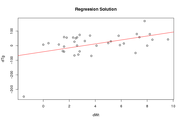
| Title produced by software | Simple Linear Regression | ||||||||||||||||||||||||||||||||||||||||||||||||||||||||||||||||||||||||||||||||||||||||||||||||||||||||||||||||||||||||||||||||||||||||||||||||||||||||||||||||||||||||
| Date of computation | Fri, 04 May 2012 15:33:41 -0400 | ||||||||||||||||||||||||||||||||||||||||||||||||||||||||||||||||||||||||||||||||||||||||||||||||||||||||||||||||||||||||||||||||||||||||||||||||||||||||||||||||||||||||
| Cite this page as follows | Statistical Computations at FreeStatistics.org, Office for Research Development and Education, URL https://freestatistics.org/blog/index.php?v=date/2012/May/04/t1336160126kbv853keenejdp9.htm/, Retrieved Fri, 03 May 2024 14:47:57 +0000 | ||||||||||||||||||||||||||||||||||||||||||||||||||||||||||||||||||||||||||||||||||||||||||||||||||||||||||||||||||||||||||||||||||||||||||||||||||||||||||||||||||||||||
| Statistical Computations at FreeStatistics.org, Office for Research Development and Education, URL https://freestatistics.org/blog/index.php?pk=166214, Retrieved Fri, 03 May 2024 14:47:57 +0000 | |||||||||||||||||||||||||||||||||||||||||||||||||||||||||||||||||||||||||||||||||||||||||||||||||||||||||||||||||||||||||||||||||||||||||||||||||||||||||||||||||||||||||
| QR Codes: | |||||||||||||||||||||||||||||||||||||||||||||||||||||||||||||||||||||||||||||||||||||||||||||||||||||||||||||||||||||||||||||||||||||||||||||||||||||||||||||||||||||||||
|
| |||||||||||||||||||||||||||||||||||||||||||||||||||||||||||||||||||||||||||||||||||||||||||||||||||||||||||||||||||||||||||||||||||||||||||||||||||||||||||||||||||||||||
| Original text written by user: | |||||||||||||||||||||||||||||||||||||||||||||||||||||||||||||||||||||||||||||||||||||||||||||||||||||||||||||||||||||||||||||||||||||||||||||||||||||||||||||||||||||||||
| IsPrivate? | No (this computation is public) | ||||||||||||||||||||||||||||||||||||||||||||||||||||||||||||||||||||||||||||||||||||||||||||||||||||||||||||||||||||||||||||||||||||||||||||||||||||||||||||||||||||||||
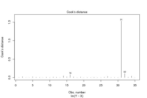
| User-defined keywords | regression, triglyceride, Cook's distance | ||||||||||||||||||||||||||||||||||||||||||||||||||||||||||||||||||||||||||||||||||||||||||||||||||||||||||||||||||||||||||||||||||||||||||||||||||||||||||||||||||||||||
| Estimated Impact | 259 | ||||||||||||||||||||||||||||||||||||||||||||||||||||||||||||||||||||||||||||||||||||||||||||||||||||||||||||||||||||||||||||||||||||||||||||||||||||||||||||||||||||||||
Tree of Dependent Computations | |||||||||||||||||||||||||||||||||||||||||||||||||||||||||||||||||||||||||||||||||||||||||||||||||||||||||||||||||||||||||||||||||||||||||||||||||||||||||||||||||||||||||
| Family? (F = Feedback message, R = changed R code, M = changed R Module, P = changed Parameters, D = changed Data) | |||||||||||||||||||||||||||||||||||||||||||||||||||||||||||||||||||||||||||||||||||||||||||||||||||||||||||||||||||||||||||||||||||||||||||||||||||||||||||||||||||||||||
| - [Simple Linear Regression] [Triglyceridge Reg...] [2011-07-07 15:11:49] [74be16979710d4c4e7c6647856088456] - R [Simple Linear Regression] [Triglyceride] [2012-05-04 19:33:41] [a9208f4f8d3b118336aae915785f2bd9] [Current] - R PD [Simple Linear Regression] [Weight and repwt] [2012-05-18 10:23:29] [7ea38fd282b91216ab82daacee092d04] - R D [Simple Linear Regression] [Height and report...] [2012-05-18 10:36:47] [7ea38fd282b91216ab82daacee092d04] - RMPD [Correlation] [Weight and rwpwt] [2012-05-18 10:46:18] [7ea38fd282b91216ab82daacee092d04] - R D [Correlation] [height and repht] [2012-05-18 10:55:24] [7ea38fd282b91216ab82daacee092d04] - PD [Simple Linear Regression] [Height and Repht] [2012-05-18 10:37:26] [57024cd1b86b0c927abdd12956d76b30] - RMPD [Correlation] [correlations - Pe...] [2012-05-18 10:46:55] [57024cd1b86b0c927abdd12956d76b30] - RMPD [Correlation] [ Correlations- He...] [2012-05-18 10:51:28] [57024cd1b86b0c927abdd12956d76b30] - PD [Simple Linear Regression] [Height and Repht ] [2012-05-18 12:12:11] [57024cd1b86b0c927abdd12956d76b30] - PD [Simple Linear Regression] [weight and repwt ...] [2012-05-18 12:17:01] [57024cd1b86b0c927abdd12956d76b30] - RM [Simple Linear Regression] [practice] [2012-05-27 18:58:23] [74be16979710d4c4e7c6647856088456] - RMP [Simple Linear Regression] [] [2012-05-31 14:30:42] [9fd651d676601517bf05777b8cc41305] - R [Simple Linear Regression] [Regression analys...] [2012-06-01 08:34:37] [e3bca26b0e60ee0c7c12e4668b30341a] - R [Simple Linear Regression] [Linear Regression...] [2012-06-01 08:34:50] [553711af6a3a99aac240956ee7ba8417] - RM [Simple Linear Regression] [diagrams for line...] [2012-06-01 08:36:00] [113a1c41b2127daa39468f799d579e88] - R [Simple Linear Regression] [Triglyceride and ...] [2012-06-01 08:36:44] [1df59b033a8a389fe796882308e19ea7] - RM [Simple Linear Regression] [q1] [2012-06-01 08:38:21] [1f171d1ca9c2c46c2a686cab36883fde] - RM [Simple Linear Regression] [] [2012-06-01 08:40:44] [d55122ee5e044ecdc19d88efcb3e2fa2] - RM [Simple Linear Regression] [i11] [2012-06-01 08:40:34] [1f171d1ca9c2c46c2a686cab36883fde] - RM [Simple Linear Regression] [regression model] [2012-06-01 08:40:42] [1a620483555ed9c2c7b5616febb12cf1] - RM [Simple Linear Regression] [A1] [2012-06-01 08:41:53] [d39358af01c9a38e48e5763b6366a442] - RM [Simple Linear Regression] [Regression] [2012-06-01 08:41:37] [e1b7a214c35f3dd75b27bf506e4bc4a9] - RM [Simple Linear Regression] [exam q1a] [2012-06-01 08:42:53] [dad037f44fabfe86d5fbc624d8e4b058] - RM [Simple Linear Regression] [] [2012-06-01 08:42:41] [b21bb0d9202f9e6611c4c3139bfbacb6] - RM [Simple Linear Regression] [] [2012-06-01 08:43:10] [1a620483555ed9c2c7b5616febb12cf1] - RM [Simple Linear Regression] [Linear Regression] [2012-06-01 08:43:20] [1e1c1716e76900be3ca46668df52a341] - R [Simple Linear Regression] [Triglyceridge and...] [2012-06-01 08:43:08] [221b3b4216f0c3837d81a9a9f89ff273] - RM [Simple Linear Regression] [Linear regression...] [2012-06-01 08:41:39] [ac59e217462c4b907248e97ba2ac8ba3] - RM [Simple Linear Regression] [] [2012-06-01 08:44:50] [6920cf7129d32b5e1d3344311b2c82d4] - R [Simple Linear Regression] [] [2012-06-01 08:44:59] [fd462f79e8628260c1cdaa3badd3b070] - RM [Simple Linear Regression] [Relationship betw...] [2012-06-01 08:44:43] [1bd8d3e7b11d3e986b30388f410fa8ef] - RM [Simple Linear Regression] [] [2012-06-01 08:45:31] [6920cf7129d32b5e1d3344311b2c82d4] - RM [Simple Linear Regression] [] [2012-06-01 08:37:00] [6d70bcb4b0f66de2508b3c69559959a1] - RM [Simple Linear Regression] [] [2012-06-01 08:45:56] [4d6fcff7a029721f667cce838c3bc5ec] - R [Simple Linear Regression] [weight and tg] [2012-06-01 08:45:15] [fe0c9d87cf8fab75feea5259b25a6bc4] - RM [Simple Linear Regression] [q1b1] [2012-06-01 08:46:33] [bebda4761be1c043611119379a4f9d90] - R [Simple Linear Regression] [ExamRegression] [2012-06-01 08:46:39] [803f089ae787812348a044658060aefb] - RM [Simple Linear Regression] [regresssion] [2012-06-01 08:46:48] [c7597844baaca9882f0ad96a032255a8] - PD [Simple Linear Regression] [new regression li...] [2012-06-01 08:46:55] [113a1c41b2127daa39468f799d579e88] - RM [Simple Linear Regression] [Relationship betw...] [2012-06-01 08:47:08] [1bd8d3e7b11d3e986b30388f410fa8ef] - R [Simple Linear Regression] [Weight loss and T...] [2012-06-01 08:45:07] [b7df83e0fc4d05ddde076a5a0ec0675f] - D [Simple Linear Regression] [Weight loss and T...] [2012-06-01 09:13:34] [b7df83e0fc4d05ddde076a5a0ec0675f] - RMPD [Kolmogorov-Smirnov Test] [Mens and Women we...] [2012-06-01 09:56:14] [b7df83e0fc4d05ddde076a5a0ec0675f] - RMPD [T-Tests] [True weight and s...] [2012-06-01 10:22:44] [b7df83e0fc4d05ddde076a5a0ec0675f] - RMPD [T-Tests] [True weight and s...] [2012-06-01 10:24:50] [b7df83e0fc4d05ddde076a5a0ec0675f] - RM [Simple Linear Regression] [] [2012-06-01 08:47:45] [a63c53a5ffd62668590cfb76aad837c1] - R [Simple Linear Regression] [exam regression] [2012-06-01 08:47:54] [57084a6890c0bc671c16163e98194e4e] - R [Simple Linear Regression] [Tricglyceride vs ...] [2012-06-01 08:48:24] [ac59e217462c4b907248e97ba2ac8ba3] - R PD [Simple Linear Regression] [Weight against re...] [2012-06-01 09:31:32] [ac59e217462c4b907248e97ba2ac8ba3] [Truncated] | |||||||||||||||||||||||||||||||||||||||||||||||||||||||||||||||||||||||||||||||||||||||||||||||||||||||||||||||||||||||||||||||||||||||||||||||||||||||||||||||||||||||||
| Feedback Forum | |||||||||||||||||||||||||||||||||||||||||||||||||||||||||||||||||||||||||||||||||||||||||||||||||||||||||||||||||||||||||||||||||||||||||||||||||||||||||||||||||||||||||
Post a new message | |||||||||||||||||||||||||||||||||||||||||||||||||||||||||||||||||||||||||||||||||||||||||||||||||||||||||||||||||||||||||||||||||||||||||||||||||||||||||||||||||||||||||
Dataset | |||||||||||||||||||||||||||||||||||||||||||||||||||||||||||||||||||||||||||||||||||||||||||||||||||||||||||||||||||||||||||||||||||||||||||||||||||||||||||||||||||||||||
| Dataseries X: | |||||||||||||||||||||||||||||||||||||||||||||||||||||||||||||||||||||||||||||||||||||||||||||||||||||||||||||||||||||||||||||||||||||||||||||||||||||||||||||||||||||||||
1.6 -41.0 1.8 55.0 5.2 30.0 4.1 0.0 0.4 17.0 2.7 -61.0 2.4 27.0 2.6 1.0 2.4 -67.0 7.2 80.0 3.7 -70.0 8.4 41.0 1.5 -37.0 8.0 0.0 0.0 7.0 7.1 -50.0 2.8 74.0 8.2 79.0 2.3 56.0 5.0 18.0 5.9 4.0 6.2 15.0 3.6 69.0 1.6 -6.0 3.2 32.0 2.6 57.0 1.6 59.0 5.8 68.0 2.8 -39.0 1.2 8.0 -1.5 -349.0 7.8 169.0 2.5 51.0 9.6 43.0 7.4 58.0 | |||||||||||||||||||||||||||||||||||||||||||||||||||||||||||||||||||||||||||||||||||||||||||||||||||||||||||||||||||||||||||||||||||||||||||||||||||||||||||||||||||||||||
Tables (Output of Computation) | |||||||||||||||||||||||||||||||||||||||||||||||||||||||||||||||||||||||||||||||||||||||||||||||||||||||||||||||||||||||||||||||||||||||||||||||||||||||||||||||||||||||||
| |||||||||||||||||||||||||||||||||||||||||||||||||||||||||||||||||||||||||||||||||||||||||||||||||||||||||||||||||||||||||||||||||||||||||||||||||||||||||||||||||||||||||
Figures (Output of Computation) | |||||||||||||||||||||||||||||||||||||||||||||||||||||||||||||||||||||||||||||||||||||||||||||||||||||||||||||||||||||||||||||||||||||||||||||||||||||||||||||||||||||||||
Input Parameters & R Code | |||||||||||||||||||||||||||||||||||||||||||||||||||||||||||||||||||||||||||||||||||||||||||||||||||||||||||||||||||||||||||||||||||||||||||||||||||||||||||||||||||||||||
| Parameters (Session): | |||||||||||||||||||||||||||||||||||||||||||||||||||||||||||||||||||||||||||||||||||||||||||||||||||||||||||||||||||||||||||||||||||||||||||||||||||||||||||||||||||||||||
| par1 = 2 ; par2 = 1 ; par3 = TRUE ; | |||||||||||||||||||||||||||||||||||||||||||||||||||||||||||||||||||||||||||||||||||||||||||||||||||||||||||||||||||||||||||||||||||||||||||||||||||||||||||||||||||||||||
| Parameters (R input): | |||||||||||||||||||||||||||||||||||||||||||||||||||||||||||||||||||||||||||||||||||||||||||||||||||||||||||||||||||||||||||||||||||||||||||||||||||||||||||||||||||||||||
| par1 = 2 ; par2 = 1 ; par3 = TRUE ; | |||||||||||||||||||||||||||||||||||||||||||||||||||||||||||||||||||||||||||||||||||||||||||||||||||||||||||||||||||||||||||||||||||||||||||||||||||||||||||||||||||||||||
| R code (references can be found in the software module): | |||||||||||||||||||||||||||||||||||||||||||||||||||||||||||||||||||||||||||||||||||||||||||||||||||||||||||||||||||||||||||||||||||||||||||||||||||||||||||||||||||||||||
cat1 <- as.numeric(par1) | |||||||||||||||||||||||||||||||||||||||||||||||||||||||||||||||||||||||||||||||||||||||||||||||||||||||||||||||||||||||||||||||||||||||||||||||||||||||||||||||||||||||||