Free Statistics
of Irreproducible Research!
Description of Statistical Computation | |||||||||||||||||||||||||||||||||||||||||||||||||||||||||||||||||
|---|---|---|---|---|---|---|---|---|---|---|---|---|---|---|---|---|---|---|---|---|---|---|---|---|---|---|---|---|---|---|---|---|---|---|---|---|---|---|---|---|---|---|---|---|---|---|---|---|---|---|---|---|---|---|---|---|---|---|---|---|---|---|---|---|---|
| Author's title | |||||||||||||||||||||||||||||||||||||||||||||||||||||||||||||||||
| Author | *The author of this computation has been verified* | ||||||||||||||||||||||||||||||||||||||||||||||||||||||||||||||||
| R Software Module | rwasp_Tests to Compare Two Means.wasp | ||||||||||||||||||||||||||||||||||||||||||||||||||||||||||||||||
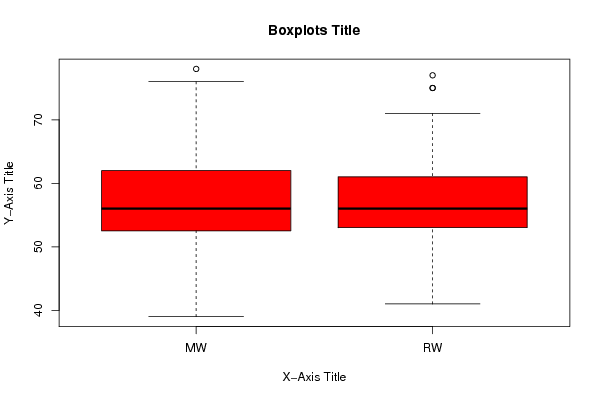
| Title produced by software | T-Tests | ||||||||||||||||||||||||||||||||||||||||||||||||||||||||||||||||
| Date of computation | Fri, 01 Jun 2012 06:11:55 -0400 | ||||||||||||||||||||||||||||||||||||||||||||||||||||||||||||||||
| Cite this page as follows | Statistical Computations at FreeStatistics.org, Office for Research Development and Education, URL https://freestatistics.org/blog/index.php?v=date/2012/Jun/01/t1338545539vybwqaacgg01r8y.htm/, Retrieved Wed, 01 May 2024 23:15:45 +0000 | ||||||||||||||||||||||||||||||||||||||||||||||||||||||||||||||||
| Statistical Computations at FreeStatistics.org, Office for Research Development and Education, URL https://freestatistics.org/blog/index.php?pk=168594, Retrieved Wed, 01 May 2024 23:15:45 +0000 | |||||||||||||||||||||||||||||||||||||||||||||||||||||||||||||||||
| QR Codes: | |||||||||||||||||||||||||||||||||||||||||||||||||||||||||||||||||
|
| |||||||||||||||||||||||||||||||||||||||||||||||||||||||||||||||||
| Original text written by user: | |||||||||||||||||||||||||||||||||||||||||||||||||||||||||||||||||
| IsPrivate? | No (this computation is public) | ||||||||||||||||||||||||||||||||||||||||||||||||||||||||||||||||
| User-defined keywords | |||||||||||||||||||||||||||||||||||||||||||||||||||||||||||||||||
| Estimated Impact | 108 | ||||||||||||||||||||||||||||||||||||||||||||||||||||||||||||||||
Tree of Dependent Computations | |||||||||||||||||||||||||||||||||||||||||||||||||||||||||||||||||
| Family? (F = Feedback message, R = changed R code, M = changed R Module, P = changed Parameters, D = changed Data) | |||||||||||||||||||||||||||||||||||||||||||||||||||||||||||||||||
| - [Histogram, QQplot and Density] [Women measured we...] [2012-06-01 09:52:57] [b687f6e38eec57c340962174507f7a8f] - R D [Histogram, QQplot and Density] [Women reported w] [2012-06-01 09:54:56] [b687f6e38eec57c340962174507f7a8f] - D [Histogram, QQplot and Density] [women - measured ...] [2012-06-01 09:58:23] [b687f6e38eec57c340962174507f7a8f] - D [Histogram, QQplot and Density] [women reported he...] [2012-06-01 09:59:53] [b687f6e38eec57c340962174507f7a8f] - D [Histogram, QQplot and Density] [male measured ] [2012-06-01 10:01:59] [b687f6e38eec57c340962174507f7a8f] - D [Histogram, QQplot and Density] [male height measure] [2012-06-01 10:04:16] [b687f6e38eec57c340962174507f7a8f] - D [Histogram, QQplot and Density] [men reported weight] [2012-06-01 10:06:02] [b687f6e38eec57c340962174507f7a8f] - RMPD [T-Tests] [Women - measured ...] [2012-06-01 10:11:55] [088dec10f3cee2e79fb056e2eecc70f7] [Current] - R D [T-Tests] [men measured vs r...] [2012-06-01 10:15:43] [b687f6e38eec57c340962174507f7a8f] | |||||||||||||||||||||||||||||||||||||||||||||||||||||||||||||||||
| Feedback Forum | |||||||||||||||||||||||||||||||||||||||||||||||||||||||||||||||||
Post a new message | |||||||||||||||||||||||||||||||||||||||||||||||||||||||||||||||||
Dataset | |||||||||||||||||||||||||||||||||||||||||||||||||||||||||||||||||
| Dataseries X: | |||||||||||||||||||||||||||||||||||||||||||||||||||||||||||||||||
58 51 53 54 59 59 57 56 51 52 64 64 52 57 65 66 62 62 61 61 61 61 54 59 50 50 63 61 58 60 39 41 71 71 52 52 68 63 56 54 54 53 63 59 54 55 49 NA 54 56 75 75 56 57 66 65 78 75 60 59 64 63 64 62 52 51 62 61 55 54 56 57 50 50 50 NA 50 55 63 64 61 60 53 52 60 55 56 56 53 53 57 59 57 56 56 56 56 57 50 50 52 52 55 NA 55 55 47 47 45 45 62 63 53 51 52 51 57 55 64 64 59 55 55 57 76 77 62 62 68 68 55 55 52 56 47 NA 45 45 68 68 44 44 62 61 56 53 50 47 53 53 64 62 62 NA 52 53 53 55 54 55 64 66 55 55 55 55 59 55 70 67 57 58 47 47 47 45 55 NA 48 44 59 NA 58 NA 57 56 51 50 54 54 53 52 59 58 59 59 63 62 66 66 53 50 54 NA 60 NA 43 NA 63 59 56 56 60 55 58 54 50 49 59 59 51 51 62 61 | |||||||||||||||||||||||||||||||||||||||||||||||||||||||||||||||||
Tables (Output of Computation) | |||||||||||||||||||||||||||||||||||||||||||||||||||||||||||||||||
| |||||||||||||||||||||||||||||||||||||||||||||||||||||||||||||||||
Figures (Output of Computation) | |||||||||||||||||||||||||||||||||||||||||||||||||||||||||||||||||
Input Parameters & R Code | |||||||||||||||||||||||||||||||||||||||||||||||||||||||||||||||||
| Parameters (Session): | |||||||||||||||||||||||||||||||||||||||||||||||||||||||||||||||||
| par1 = two.sided ; par2 = 1 ; par3 = 2 ; par4 = T-Test ; par5 = unpaired ; par6 = 0.0 ; par7 = 0.95 ; par8 = TRUE ; | |||||||||||||||||||||||||||||||||||||||||||||||||||||||||||||||||
| Parameters (R input): | |||||||||||||||||||||||||||||||||||||||||||||||||||||||||||||||||
| par1 = two.sided ; par2 = 1 ; par3 = 2 ; par4 = T-Test ; par5 = unpaired ; par6 = 0.0 ; par7 = 0.95 ; par8 = TRUE ; | |||||||||||||||||||||||||||||||||||||||||||||||||||||||||||||||||
| R code (references can be found in the software module): | |||||||||||||||||||||||||||||||||||||||||||||||||||||||||||||||||
par2 <- as.numeric(par2) | |||||||||||||||||||||||||||||||||||||||||||||||||||||||||||||||||