Repository of Reproducible Computations

Free Statistics

of Irreproducible Research!

Author's title

Author

*Unverified author*

R Software Module

rwasp_autocorrelation.wasp

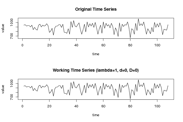
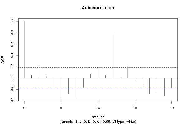
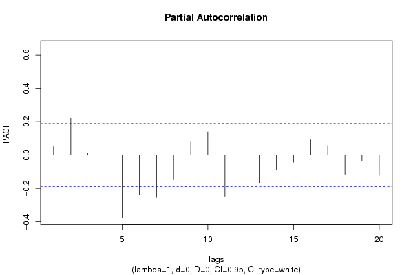
Title produced by software

(Partial) Autocorrelation Function

Date of computation

Sun, 29 Jul 2012 07:08:12 -0400

Cite this page as follows

Statistical Computations at FreeStatistics.org, Office for Research Development and Education, URL https://freestatistics.org/blog/index.php?v=date/2012/Jul/29/t1343560278gtc0x6glqbhiyfx.htm/, Retrieved Wed, 01 May 2024 22:27:27 +0000

Statistical Computations at FreeStatistics.org, Office for Research Development and Education, URL https://freestatistics.org/blog/index.php?pk=168941, Retrieved Wed, 01 May 2024 22:27:27 +0000

QR Codes:

Paste this QR Code to cite your computation.

Original text written by user:

IsPrivate?

No (this computation is public)

User-defined keywords

Bart Mortelmans

Estimated Impact

174

Family? (F = Feedback message, R = changed R code, M = changed R Module, P = changed Parameters, D = changed Data)

-     [Univariate Data Series] [Tijdreeks 2 - Stap 1] [2012-07-29 10:04:17] [f85cc8f00ef4b762f0a6fdfddc793773]
- RMP   [Harrell-Davis Quantiles] [Tijdreeks 2 - Stap 5] [2012-07-29 10:30:29] [226376a35b8869827dc57271384c00a4]
- RMP     [Mean versus Median] [Tijdreeks 2 - Stap 8] [2012-07-29 10:41:52] [226376a35b8869827dc57271384c00a4]
- RM          [(Partial) Autocorrelation Function] [Tijdreeks 2 - Sta...] [2012-07-29 11:08:12] [480fcaba71e70207c3e0ad7177944aa6] [Current]
- R             [(Partial) Autocorrelation Function] [Tijdreeks 2 - Sta...] [2012-07-29 11:12:39] [226376a35b8869827dc57271384c00a4] 
- RM            [Variability] [Tijdreeks 2 - Sta...] [2012-07-29 11:23:37] [226376a35b8869827dc57271384c00a4] 
- RM            [Standard Deviation-Mean Plot] [Tijdreeks 2 - Sta...] [2012-07-29 11:26:49] [226376a35b8869827dc57271384c00a4] 
- RM            [Classical Decomposition] [Tijdreeks 2 - Sta...] [2012-07-29 11:36:01] [226376a35b8869827dc57271384c00a4] 
- RM            [Exponential Smoothing] [Tijdreeks 2 - Sta...] [2012-07-29 11:39:43] [226376a35b8869827dc57271384c00a4] 

Feedback Forum

Post a new message

Dataseries X:

Download CSV

Histogram

Boxplots

Summary of computational transaction
Raw Input	view raw input (R code)
Raw Output	view raw output of R engine
Computing time	2 seconds
R Server	'Gwilym Jenkins' @ jenkins.wessa.net

\begin{tabular}{lllllllll}
\hline
Summary of computational transaction \tabularnewline
Raw Input & view raw input (R code)  \tabularnewline
Raw Output & view raw output of R engine  \tabularnewline
Computing time & 2 seconds \tabularnewline
R Server & 'Gwilym Jenkins' @ jenkins.wessa.net \tabularnewline
\hline
\end{tabular}
%Source: https://freestatistics.org/blog/index.php?pk=168941&T=0

[TABLE]
[ROW][C]Summary of computational transaction[/C][/ROW]
[ROW][C]Raw Input[/C][C]view raw input (R code) [/C][/ROW]
[ROW][C]Raw Output[/C][C]view raw output of R engine [/C][/ROW]
[ROW][C]Computing time[/C][C]2 seconds[/C][/ROW]
[ROW][C]R Server[/C][C]'Gwilym Jenkins' @ jenkins.wessa.net[/C][/ROW]
[/TABLE]
Source: https://freestatistics.org/blog/index.php?pk=168941&T=0

Globally Unique Identifier (entire table): ba.freestatistics.org/blog/index.php?pk=168941&T=0

As an alternative you can also use a QR Code:

The GUIDs for individual cells are displayed in the table below:

Summary of computational transaction
Raw Input	view raw input (R code)
Raw Output	view raw output of R engine
Computing time	2 seconds
R Server	'Gwilym Jenkins' @ jenkins.wessa.net

Autocorrelation Function
Time lag k	ACF(k)	T-STAT	P-value
1	0.049754	0.5171	0.303086
2	0.223512	2.3228	0.011032
3	0.02913	0.3027	0.381339
4	-0.17786	-1.8484	0.033642
5	-0.341658	-3.5506	0.000285
6	-0.279037	-2.8998	0.002262
7	-0.352349	-3.6617	0.000195
8	-0.164452	-1.709	0.045159
9	0.070546	0.7331	0.232533
10	0.175364	1.8224	0.035578
11	0.052648	0.5471	0.292707
12	0.778171	8.087	0
13	-0.010195	-0.106	0.457909
14	0.20327	2.1124	0.018476
15	-0.026025	-0.2705	0.393663
16	-0.144526	-1.502	0.068013
17	-0.282297	-2.9337	0.002046
18	-0.262412	-2.7271	0.00373
19	-0.318328	-3.3082	0.000638
20	-0.176693	-1.8362	0.034536

\begin{tabular}{lllllllll}
\hline
Autocorrelation Function \tabularnewline
Time lag k & ACF(k) & T-STAT & P-value \tabularnewline
1 & 0.049754 & 0.5171 & 0.303086 \tabularnewline
2 & 0.223512 & 2.3228 & 0.011032 \tabularnewline
3 & 0.02913 & 0.3027 & 0.381339 \tabularnewline
4 & -0.17786 & -1.8484 & 0.033642 \tabularnewline
5 & -0.341658 & -3.5506 & 0.000285 \tabularnewline
6 & -0.279037 & -2.8998 & 0.002262 \tabularnewline
7 & -0.352349 & -3.6617 & 0.000195 \tabularnewline
8 & -0.164452 & -1.709 & 0.045159 \tabularnewline
9 & 0.070546 & 0.7331 & 0.232533 \tabularnewline
10 & 0.175364 & 1.8224 & 0.035578 \tabularnewline
11 & 0.052648 & 0.5471 & 0.292707 \tabularnewline
12 & 0.778171 & 8.087 & 0 \tabularnewline
13 & -0.010195 & -0.106 & 0.457909 \tabularnewline
14 & 0.20327 & 2.1124 & 0.018476 \tabularnewline
15 & -0.026025 & -0.2705 & 0.393663 \tabularnewline
16 & -0.144526 & -1.502 & 0.068013 \tabularnewline
17 & -0.282297 & -2.9337 & 0.002046 \tabularnewline
18 & -0.262412 & -2.7271 & 0.00373 \tabularnewline
19 & -0.318328 & -3.3082 & 0.000638 \tabularnewline
20 & -0.176693 & -1.8362 & 0.034536 \tabularnewline
\hline
\end{tabular}
%Source: https://freestatistics.org/blog/index.php?pk=168941&T=1

[TABLE]
[ROW][C]Autocorrelation Function[/C][/ROW]
[ROW][C]Time lag k[/C][C]ACF(k)[/C][C]T-STAT[/C][C]P-value[/C][/ROW]
[ROW][C]1[/C][C]0.049754[/C][C]0.5171[/C][C]0.303086[/C][/ROW]
[ROW][C]2[/C][C]0.223512[/C][C]2.3228[/C][C]0.011032[/C][/ROW]
[ROW][C]3[/C][C]0.02913[/C][C]0.3027[/C][C]0.381339[/C][/ROW]
[ROW][C]4[/C][C]-0.17786[/C][C]-1.8484[/C][C]0.033642[/C][/ROW]
[ROW][C]5[/C][C]-0.341658[/C][C]-3.5506[/C][C]0.000285[/C][/ROW]
[ROW][C]6[/C][C]-0.279037[/C][C]-2.8998[/C][C]0.002262[/C][/ROW]
[ROW][C]7[/C][C]-0.352349[/C][C]-3.6617[/C][C]0.000195[/C][/ROW]
[ROW][C]8[/C][C]-0.164452[/C][C]-1.709[/C][C]0.045159[/C][/ROW]
[ROW][C]9[/C][C]0.070546[/C][C]0.7331[/C][C]0.232533[/C][/ROW]
[ROW][C]10[/C][C]0.175364[/C][C]1.8224[/C][C]0.035578[/C][/ROW]
[ROW][C]11[/C][C]0.052648[/C][C]0.5471[/C][C]0.292707[/C][/ROW]
[ROW][C]12[/C][C]0.778171[/C][C]8.087[/C][C]0[/C][/ROW]
[ROW][C]13[/C][C]-0.010195[/C][C]-0.106[/C][C]0.457909[/C][/ROW]
[ROW][C]14[/C][C]0.20327[/C][C]2.1124[/C][C]0.018476[/C][/ROW]
[ROW][C]15[/C][C]-0.026025[/C][C]-0.2705[/C][C]0.393663[/C][/ROW]
[ROW][C]16[/C][C]-0.144526[/C][C]-1.502[/C][C]0.068013[/C][/ROW]
[ROW][C]17[/C][C]-0.282297[/C][C]-2.9337[/C][C]0.002046[/C][/ROW]
[ROW][C]18[/C][C]-0.262412[/C][C]-2.7271[/C][C]0.00373[/C][/ROW]
[ROW][C]19[/C][C]-0.318328[/C][C]-3.3082[/C][C]0.000638[/C][/ROW]
[ROW][C]20[/C][C]-0.176693[/C][C]-1.8362[/C][C]0.034536[/C][/ROW]
[/TABLE]
Source: https://freestatistics.org/blog/index.php?pk=168941&T=1

Globally Unique Identifier (entire table): ba.freestatistics.org/blog/index.php?pk=168941&T=1

As an alternative you can also use a QR Code:

The GUIDs for individual cells are displayed in the table below:

Autocorrelation Function
Time lag k	ACF(k)	T-STAT	P-value
1	0.049754	0.5171	0.303086
2	0.223512	2.3228	0.011032
3	0.02913	0.3027	0.381339
4	-0.17786	-1.8484	0.033642
5	-0.341658	-3.5506	0.000285
6	-0.279037	-2.8998	0.002262
7	-0.352349	-3.6617	0.000195
8	-0.164452	-1.709	0.045159
9	0.070546	0.7331	0.232533
10	0.175364	1.8224	0.035578
11	0.052648	0.5471	0.292707
12	0.778171	8.087	0
13	-0.010195	-0.106	0.457909
14	0.20327	2.1124	0.018476
15	-0.026025	-0.2705	0.393663
16	-0.144526	-1.502	0.068013
17	-0.282297	-2.9337	0.002046
18	-0.262412	-2.7271	0.00373
19	-0.318328	-3.3082	0.000638
20	-0.176693	-1.8362	0.034536

Partial Autocorrelation Function
Time lag k	PACF(k)	T-STAT	P-value
1	0.049754	0.5171	0.303086
2	0.221585	2.3028	0.011604
3	0.009962	0.1035	0.45887
4	-0.241299	-2.5076	0.006821
5	-0.374958	-3.8967	8.5e-05
6	-0.235501	-2.4474	0.008001
7	-0.253409	-2.6335	0.004845
8	-0.147288	-1.5307	0.064389
9	0.082455	0.8569	0.196699
10	0.138114	1.4353	0.077043
11	-0.24666	-2.5634	0.005871
12	0.645784	6.7112	0
13	-0.165401	-1.7189	0.044249
14	-0.090992	-0.9456	0.173227
15	-0.04331	-0.4501	0.326775
16	0.094848	0.9857	0.163244
17	0.057329	0.5958	0.276285
18	-0.115069	-1.1958	0.11719
19	-0.032747	-0.3403	0.367138
20	-0.122025	-1.2681	0.10374

\begin{tabular}{lllllllll}
\hline
Partial Autocorrelation Function \tabularnewline
Time lag k & PACF(k) & T-STAT & P-value \tabularnewline
1 & 0.049754 & 0.5171 & 0.303086 \tabularnewline
2 & 0.221585 & 2.3028 & 0.011604 \tabularnewline
3 & 0.009962 & 0.1035 & 0.45887 \tabularnewline
4 & -0.241299 & -2.5076 & 0.006821 \tabularnewline
5 & -0.374958 & -3.8967 & 8.5e-05 \tabularnewline
6 & -0.235501 & -2.4474 & 0.008001 \tabularnewline
7 & -0.253409 & -2.6335 & 0.004845 \tabularnewline
8 & -0.147288 & -1.5307 & 0.064389 \tabularnewline
9 & 0.082455 & 0.8569 & 0.196699 \tabularnewline
10 & 0.138114 & 1.4353 & 0.077043 \tabularnewline
11 & -0.24666 & -2.5634 & 0.005871 \tabularnewline
12 & 0.645784 & 6.7112 & 0 \tabularnewline
13 & -0.165401 & -1.7189 & 0.044249 \tabularnewline
14 & -0.090992 & -0.9456 & 0.173227 \tabularnewline
15 & -0.04331 & -0.4501 & 0.326775 \tabularnewline
16 & 0.094848 & 0.9857 & 0.163244 \tabularnewline
17 & 0.057329 & 0.5958 & 0.276285 \tabularnewline
18 & -0.115069 & -1.1958 & 0.11719 \tabularnewline
19 & -0.032747 & -0.3403 & 0.367138 \tabularnewline
20 & -0.122025 & -1.2681 & 0.10374 \tabularnewline
\hline
\end{tabular}
%Source: https://freestatistics.org/blog/index.php?pk=168941&T=2

[TABLE]
[ROW][C]Partial Autocorrelation Function[/C][/ROW]
[ROW][C]Time lag k[/C][C]PACF(k)[/C][C]T-STAT[/C][C]P-value[/C][/ROW]
[ROW][C]1[/C][C]0.049754[/C][C]0.5171[/C][C]0.303086[/C][/ROW]
[ROW][C]2[/C][C]0.221585[/C][C]2.3028[/C][C]0.011604[/C][/ROW]
[ROW][C]3[/C][C]0.009962[/C][C]0.1035[/C][C]0.45887[/C][/ROW]
[ROW][C]4[/C][C]-0.241299[/C][C]-2.5076[/C][C]0.006821[/C][/ROW]
[ROW][C]5[/C][C]-0.374958[/C][C]-3.8967[/C][C]8.5e-05[/C][/ROW]
[ROW][C]6[/C][C]-0.235501[/C][C]-2.4474[/C][C]0.008001[/C][/ROW]
[ROW][C]7[/C][C]-0.253409[/C][C]-2.6335[/C][C]0.004845[/C][/ROW]
[ROW][C]8[/C][C]-0.147288[/C][C]-1.5307[/C][C]0.064389[/C][/ROW]
[ROW][C]9[/C][C]0.082455[/C][C]0.8569[/C][C]0.196699[/C][/ROW]
[ROW][C]10[/C][C]0.138114[/C][C]1.4353[/C][C]0.077043[/C][/ROW]
[ROW][C]11[/C][C]-0.24666[/C][C]-2.5634[/C][C]0.005871[/C][/ROW]
[ROW][C]12[/C][C]0.645784[/C][C]6.7112[/C][C]0[/C][/ROW]
[ROW][C]13[/C][C]-0.165401[/C][C]-1.7189[/C][C]0.044249[/C][/ROW]
[ROW][C]14[/C][C]-0.090992[/C][C]-0.9456[/C][C]0.173227[/C][/ROW]
[ROW][C]15[/C][C]-0.04331[/C][C]-0.4501[/C][C]0.326775[/C][/ROW]
[ROW][C]16[/C][C]0.094848[/C][C]0.9857[/C][C]0.163244[/C][/ROW]
[ROW][C]17[/C][C]0.057329[/C][C]0.5958[/C][C]0.276285[/C][/ROW]
[ROW][C]18[/C][C]-0.115069[/C][C]-1.1958[/C][C]0.11719[/C][/ROW]
[ROW][C]19[/C][C]-0.032747[/C][C]-0.3403[/C][C]0.367138[/C][/ROW]
[ROW][C]20[/C][C]-0.122025[/C][C]-1.2681[/C][C]0.10374[/C][/ROW]
[/TABLE]
Source: https://freestatistics.org/blog/index.php?pk=168941&T=2

Globally Unique Identifier (entire table): ba.freestatistics.org/blog/index.php?pk=168941&T=2

As an alternative you can also use a QR Code:

The GUIDs for individual cells are displayed in the table below:

Partial Autocorrelation Function
Time lag k	PACF(k)	T-STAT	P-value
1	0.049754	0.5171	0.303086
2	0.221585	2.3028	0.011604
3	0.009962	0.1035	0.45887
4	-0.241299	-2.5076	0.006821
5	-0.374958	-3.8967	8.5e-05
6	-0.235501	-2.4474	0.008001
7	-0.253409	-2.6335	0.004845
8	-0.147288	-1.5307	0.064389
9	0.082455	0.8569	0.196699
10	0.138114	1.4353	0.077043
11	-0.24666	-2.5634	0.005871
12	0.645784	6.7112	0
13	-0.165401	-1.7189	0.044249
14	-0.090992	-0.9456	0.173227
15	-0.04331	-0.4501	0.326775
16	0.094848	0.9857	0.163244
17	0.057329	0.5958	0.276285
18	-0.115069	-1.1958	0.11719
19	-0.032747	-0.3403	0.367138
20	-0.122025	-1.2681	0.10374

Figure 1

PNG link

Postscript link

PDF link

Figure 2

PNG link

Postscript link

PDF link

Figure 3

PNG link

Postscript link

PDF link

Parameters (Session):

par1 = 0.01 ; par2 = 0.99 ; par3 = 0.01 ;

Parameters (R input):

par1 = Default ; par2 = 1 ; par3 = 0 ; par4 = 0 ; par5 = 12 ; par6 = White Noise ; par7 = 0.95 ; par8 = ;

R code (references can be found in the software module):

if (par1 == 'Default') {
par1 = 10*log10(length(x))
} else {
par1 <- as.numeric(par1)
}
par2 <- as.numeric(par2)
par3 <- as.numeric(par3)
par4 <- as.numeric(par4)
par5 <- as.numeric(par5)
if (par6 == 'White Noise') par6 <- 'white' else par6 <- 'ma'
par7 <- as.numeric(par7)
if (par8 != '') par8 <- as.numeric(par8)
ox <- x
if (par8 == '') {
if (par2 == 0) {
x <- log(x)
} else {
x <- (x ^ par2 - 1) / par2
}
} else {
x <- log(x,base=par8)
}
if (par3 > 0) x <- diff(x,lag=1,difference=par3)
if (par4 > 0) x <- diff(x,lag=par5,difference=par4)
bitmap(file='picts.png')
op <- par(mfrow=c(2,1))
plot(ox,type='l',main='Original Time Series',xlab='time',ylab='value')
if (par8=='') {
mytitle <- paste('Working Time Series (lambda=',par2,', d=',par3,', D=',par4,')',sep='')
mysub <- paste('(lambda=',par2,', d=',par3,', D=',par4,', CI=', par7, ', CI type=',par6,')',sep='')
} else {
mytitle <- paste('Working Time Series (base=',par8,', d=',par3,', D=',par4,')',sep='')
mysub <- paste('(base=',par8,', d=',par3,', D=',par4,', CI=', par7, ', CI type=',par6,')',sep='')
}
plot(x,type='l', main=mytitle,xlab='time',ylab='value')
par(op)
dev.off()
bitmap(file='pic1.png')
racf <- acf(x, par1, main='Autocorrelation', xlab='time lag', ylab='ACF', ci.type=par6, ci=par7, sub=mysub)
dev.off()
bitmap(file='pic2.png')
rpacf <- pacf(x,par1,main='Partial Autocorrelation',xlab='lags',ylab='PACF',sub=mysub)
dev.off()
(myacf <- c(racf$acf))
(mypacf <- c(rpacf$acf))
lengthx <- length(x)
sqrtn <- sqrt(lengthx)
load(file='createtable')
a<-table.start()
a<-table.row.start(a)
a<-table.element(a,'Autocorrelation Function',4,TRUE)
a<-table.row.end(a)
a<-table.row.start(a)
a<-table.element(a,'Time lag k',header=TRUE)
a<-table.element(a,hyperlink('basics.htm','ACF(k)','click here for more information about the Autocorrelation Function'),header=TRUE)
a<-table.element(a,'T-STAT',header=TRUE)
a<-table.element(a,'P-value',header=TRUE)
a<-table.row.end(a)
for (i in 2:(par1+1)) {
a<-table.row.start(a)
a<-table.element(a,i-1,header=TRUE)
a<-table.element(a,round(myacf[i],6))
mytstat <- myacf[i]*sqrtn
a<-table.element(a,round(mytstat,4))
a<-table.element(a,round(1-pt(abs(mytstat),lengthx),6))
a<-table.row.end(a)
}
a<-table.end(a)
table.save(a,file='mytable.tab')
a<-table.start()
a<-table.row.start(a)
a<-table.element(a,'Partial Autocorrelation Function',4,TRUE)
a<-table.row.end(a)
a<-table.row.start(a)
a<-table.element(a,'Time lag k',header=TRUE)
a<-table.element(a,hyperlink('basics.htm','PACF(k)','click here for more information about the Partial Autocorrelation Function'),header=TRUE)
a<-table.element(a,'T-STAT',header=TRUE)
a<-table.element(a,'P-value',header=TRUE)
a<-table.row.end(a)
for (i in 1:par1) {
a<-table.row.start(a)
a<-table.element(a,i,header=TRUE)
a<-table.element(a,round(mypacf[i],6))
mytstat <- mypacf[i]*sqrtn
a<-table.element(a,round(mytstat,4))
a<-table.element(a,round(1-pt(abs(mytstat),lengthx),6))
a<-table.row.end(a)
}
a<-table.end(a)
table.save(a,file='mytable1.tab')

Free Statistics

Description of Statistical Computation

Tree of Dependent Computations

Dataset

Tables (Output of Computation)

Figures (Output of Computation)

Input Parameters & R Code