Free Statistics
of Irreproducible Research!
Description of Statistical Computation | |||||||||||||||||||||
|---|---|---|---|---|---|---|---|---|---|---|---|---|---|---|---|---|---|---|---|---|---|
| Author's title | |||||||||||||||||||||
| Author | *Unverified author* | ||||||||||||||||||||
| R Software Module | rwasp_meanplot.wasp | ||||||||||||||||||||
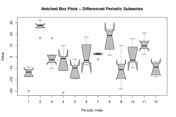
| Title produced by software | Mean Plot | ||||||||||||||||||||
| Date of computation | Sun, 15 Jan 2012 11:47:52 -0500 | ||||||||||||||||||||
| Cite this page as follows | Statistical Computations at FreeStatistics.org, Office for Research Development and Education, URL https://freestatistics.org/blog/index.php?v=date/2012/Jan/15/t1326646406luhmgfo9mcx90vy.htm/, Retrieved Fri, 03 May 2024 04:20:21 +0000 | ||||||||||||||||||||
| Statistical Computations at FreeStatistics.org, Office for Research Development and Education, URL https://freestatistics.org/blog/index.php?pk=161103, Retrieved Fri, 03 May 2024 04:20:21 +0000 | |||||||||||||||||||||
| QR Codes: | |||||||||||||||||||||
|
| |||||||||||||||||||||
| Original text written by user: | |||||||||||||||||||||
| IsPrivate? | No (this computation is public) | ||||||||||||||||||||
| User-defined keywords | KDG201162 | ||||||||||||||||||||
| Estimated Impact | 96 | ||||||||||||||||||||
Tree of Dependent Computations | |||||||||||||||||||||
| Family? (F = Feedback message, R = changed R code, M = changed R Module, P = changed Parameters, D = changed Data) | |||||||||||||||||||||
| - [Notched Boxplots] [boxplot] [2011-10-11 16:58:56] [0f3802131247472a006387bf3e5d274d] - RMPD [Mean Plot] [] [2012-01-15 16:47:52] [9bda411d6223d16f0472c7feaae49b5f] [Current] | |||||||||||||||||||||
| Feedback Forum | |||||||||||||||||||||
Post a new message | |||||||||||||||||||||
Dataset | |||||||||||||||||||||
| Dataseries X: | |||||||||||||||||||||
113,25 104,54 132,78 122,99 133,14 125,83 122,99 125,7 148,47 120,75 136,7 139,17 123,47 112,76 137,99 139,75 140,22 121,6 132,33 130,34 149,05 130,47 139,29 146,55 137,79 122,95 139,51 155,77 143,95 125,07 142,35 144,34 145,87 156,01 146,74 156,45 152,29 122,56 154,59 149,68 118,75 109,22 104,19 107,33 114,07 107,92 103,53 117,3 112,09 95,08 123,28 121,98 121,74 119,93 113,31 117,19 141,13 130,18 127,47 148,33 131,24 119,99 146,49 142,98 140,65 131,15 | |||||||||||||||||||||
Tables (Output of Computation) | |||||||||||||||||||||
| |||||||||||||||||||||
Figures (Output of Computation) | |||||||||||||||||||||
Input Parameters & R Code | |||||||||||||||||||||
| Parameters (Session): | |||||||||||||||||||||
| Parameters (R input): | |||||||||||||||||||||
| par1 = 12 ; | |||||||||||||||||||||
| R code (references can be found in the software module): | |||||||||||||||||||||
par1 <- as.numeric(par1) | |||||||||||||||||||||