Repository of Reproducible Computations

Free Statistics

of Irreproducible Research!

Author's title

Author

*The author of this computation has been verified*

R Software Module

rwasp_Tests to Compare Two Means.wasp

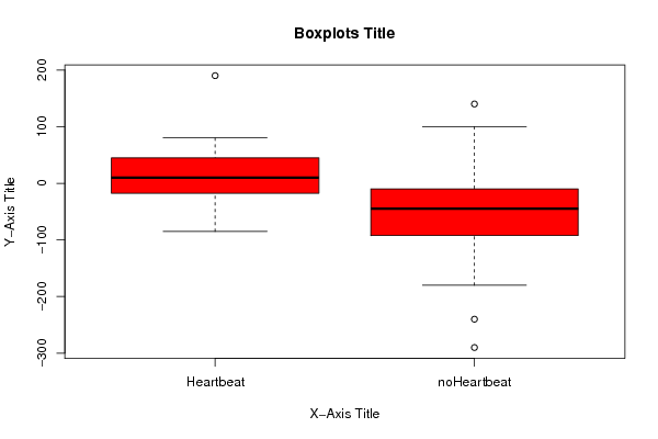
Title produced by software

T-Tests

Date of computation

Tue, 14 Feb 2012 11:56:38 -0500

Cite this page as follows

Statistical Computations at FreeStatistics.org, Office for Research Development and Education, URL https://freestatistics.org/blog/index.php?v=date/2012/Feb/14/t13292387940gxd5coql7uku3s.htm/, Retrieved Mon, 29 Apr 2024 14:30:46 +0000

Statistical Computations at FreeStatistics.org, Office for Research Development and Education, URL https://freestatistics.org/blog/index.php?pk=162316, Retrieved Mon, 29 Apr 2024 14:30:46 +0000

QR Codes:

Paste this QR Code to cite your computation.

Original text written by user:

IsPrivate?

No (this computation is public)

User-defined keywords

Estimated Impact

166

Family? (F = Feedback message, R = changed R code, M = changed R Module, P = changed Parameters, D = changed Data)

-       [T-Tests] [Salk Heatbeat Study] [2012-02-14 16:56:38] [a9208f4f8d3b118336aae915785f2bd9] [Current]
- R       [T-Tests] [Salk Heatbeat Study] [2012-02-14 17:06:34] [98fd0e87c3eb04e0cc2efde01dbafab6] 
- RMPD    [Histogram, QQplot and Density] [Salk Heatbeat Stu...] [2012-02-14 17:58:15] [98fd0e87c3eb04e0cc2efde01dbafab6] 
- RMP       [Histogram, QQplot and Density] [qq plot] [2012-05-03 09:19:25] [ea6e45d26e44fca6fcec5c603ff1140c] 
- R P       [Histogram, QQplot and Density] [No heartbeat ] [2012-05-03 09:19:54] [35521cdb85a31d9f6eb48e92142bc928] 
- R P       [Histogram, QQplot and Density] [NoHBSample] [2012-05-03 09:21:32] [5af04e13c06bbf1f7fb207eb9550d664] 
-             [Histogram, QQplot and Density] [NoHB] [2012-05-03 09:25:27] [5af04e13c06bbf1f7fb207eb9550d664] 
- RMP       [Histogram, QQplot and Density] [qqplot] [2012-05-03 09:21:53] [c2d7eae68f5ec0337d2d2ba826377ba0] 
- RMP       [Histogram, QQplot and Density] [grpahs for no hea...] [2012-05-03 09:23:04] [c2d7eae68f5ec0337d2d2ba826377ba0] 
- R P       [Histogram, QQplot and Density] [no heartbeat] [2012-05-03 09:25:25] [35521cdb85a31d9f6eb48e92142bc928] 
- R P       [Histogram, QQplot and Density] [] [2012-05-03 09:26:08] [2d5cef47d6186b035b8ade2ed171f642] 
- RMP       [Histogram, QQplot and Density] [] [2012-05-03 09:29:38] [2d5cef47d6186b035b8ade2ed171f642] 
- RMP       [Histogram and QQplot] [] [2012-05-03 09:29:58] [74be16979710d4c4e7c6647856088456] 
- RMP       [Histogram, QQplot and Density] [no heartbeat] [2012-05-03 09:33:10] [c2d7eae68f5ec0337d2d2ba826377ba0] 
- R P       [Histogram, QQplot and Density] [20 bins ] [2012-05-03 09:35:40] [bf1ddb3cd45fb5d723b760bc40755ff6] 
- R P       [Histogram, QQplot and Density] [Graph one] [2012-05-03 09:38:03] [57084a6890c0bc671c16163e98194e4e] 
- RMP       [Histogram, QQplot and Density] [no heartbeat] [2012-05-03 09:37:41] [dcbd67829fb198dc024d653d5871c807] 
- RMP       [Histogram, QQplot and Density] [Box Plot 1 ] [2012-05-03 09:39:21] [f5d7ef0e9b68469df85069f757ece0ab] 
- R P       [Histogram, QQplot and Density] [No heartbeat] [2012-05-03 09:39:22] [1bd8d3e7b11d3e986b30388f410fa8ef] 
- R P       [Histogram, QQplot and Density] [Babies not expose...] [2012-05-03 09:40:00] [b7df83e0fc4d05ddde076a5a0ec0675f] 
- RMP       [Histogram, QQplot and Density] [Plots For No Hear...] [2012-05-03 09:40:01] [9a61272a736950814aceafb9bfc5e47e] 
- RMP       [Histogram, QQplot and Density] [Distributional pl...] [2012-05-03 09:39:58] [a68359a26e24fd92b609f4c95c254176] 
- RMP       [Histogram, QQplot and Density] [Descriptive Stati...] [2012-05-03 09:40:19] [09253b89c68efd7a460a267273a9d6e3] 
- RMP       [Histogram, QQplot and Density] [] [2012-05-03 09:41:11] [a63c53a5ffd62668590cfb76aad837c1] 
- R P       [Histogram, QQplot and Density] [Graph one] [2012-05-03 09:41:22] [57084a6890c0bc671c16163e98194e4e] 
- RMP       [Histogram, QQplot and Density] [Box  Plot 1 ] [2012-05-03 09:41:37] [f5d7ef0e9b68469df85069f757ece0ab] 
- RMP       [Histogram, QQplot and Density] [graphs to represe...] [2012-05-03 09:42:34] [04881406e92e7b483917daebdd502463] 
- RMP       [Histogram, QQplot and Density] [Box Plot 1] [2012-05-03 09:42:39] [f5d7ef0e9b68469df85069f757ece0ab] 
- RMP       [Histogram, QQplot and Density] [] [2012-05-03 09:43:55] [221b3b4216f0c3837d81a9a9f89ff273] 
- RMP       [Histogram, QQplot and Density] [] [2012-05-03 09:45:58] [221b3b4216f0c3837d81a9a9f89ff273] 
- RMP       [Histogram, QQplot and Density] [Box Plot 1 ] [2012-05-03 09:47:02] [f5d7ef0e9b68469df85069f757ece0ab] 
- R P       [Histogram, QQplot and Density] [] [2012-05-03 09:48:18] [a7ea7f4263337445a0a4c6547fb2278a] 
- R P       [Histogram, QQplot and Density] [No Heartbeat cond...] [2012-05-03 09:48:27] [5ab72825a06ca2a73c828d10c85d14d8] 
- RMP       [Histogram, QQplot and Density] [Box Plot 1] [2012-05-03 09:48:45] [f5d7ef0e9b68469df85069f757ece0ab] 
- RMPD      [Wilcoxon-Mann-Whitney Test] [Mann whitney  test] [2012-05-03 09:49:02] [57084a6890c0bc671c16163e98194e4e] 
- RMPD      [T-Tests] [A comparison of s...] [2012-05-03 09:52:21] [c14255f5a914c4d7aab5f6cd60318f9b] 
- RMPD      [T-Tests] [dgs] [2012-05-03 09:54:25] [9fd651d676601517bf05777b8cc41305] 
- RMP       [Histogram, QQplot and Density] [No heartbeat sample] [2012-05-03 09:56:35] [069c1c4384e883dd4e1df6d4e8f70f1e] 
- RMPD      [MC May Mock - Q6] [] [2012-05-30 23:07:31] [28e3b0ec23e510cd6fa92636dd93aa1d] 
- RMPD      [MC May Mock - Q6] [] [2012-05-30 23:07:31] [28e3b0ec23e510cd6fa92636dd93aa1d] 
- RMP       [Histogram, QQplot and Density] [no heartbeat sample] [2012-06-01 07:09:15] [5934aceae8cf147bda5be230722b868c] 
- R PD      [Histogram, QQplot and Density] [Summer exam] [2012-06-01 09:13:10] [8c387ce24444dc2c0e7d576cfc7658e0] 
- R PD      [Histogram, QQplot and Density] [Summer exam] [2012-06-01 09:16:53] [8c387ce24444dc2c0e7d576cfc7658e0] 
- RMPD      [Wilcoxon-Mann-Whitney Test] [Summer exam] [2012-06-01 09:29:17] [8c387ce24444dc2c0e7d576cfc7658e0] 
- RMP       [Histogram, QQplot and Density] [plot qq] [2012-08-30 09:47:14] [74be16979710d4c4e7c6647856088456] 
- R PD      [Histogram, QQplot and Density] [] [2012-08-30 10:00:56] [e5cd290daa2365fa501ea04dbf3bfa28] 
- R P       [Histogram, QQplot and Density] [Ian test] [2013-05-07 10:35:00] [98fd0e87c3eb04e0cc2efde01dbafab6] 
- RMPD      [Wilcoxon-Mann-Whitney Test] [Heartbeat vs. NoH...] [2013-05-09 09:20:45] [873a05c15549159fecd09e71c73360f4] 
- R P       [Histogram, QQplot and Density] [] [2013-05-09 09:23:58] [74be16979710d4c4e7c6647856088456] 

[Truncated]

Feedback Forum

Post a new message

Dataseries X:

Download CSV

Histogram

Boxplots

190	140
80	100
80	100
75	70
50	25
40	20
30	10
20	0
20	-10
10	-10
10	-25
10	-25
0	-25
0	-30
-10	-30
-25	-30
-30	-45
-45	-45
-60	-45
-85	-50
NA	-50
NA	-50
NA	-60
NA	-75
NA	-75
NA	-85
NA	-85
NA	-100
NA	-110
NA	-130
NA	-130
NA	-155
NA	-155
NA	-180
NA	-240
NA	-290

Summary of computational transaction
Raw Input	view raw input (R code)
Raw Output	view raw output of R engine
Computing time	1 seconds
R Server	'Gertrude Mary Cox' @ cox.wessa.net

\begin{tabular}{lllllllll}
\hline
Summary of computational transaction \tabularnewline
Raw Input & view raw input (R code)  \tabularnewline
Raw Output & view raw output of R engine  \tabularnewline
Computing time & 1 seconds \tabularnewline
R Server & 'Gertrude Mary Cox' @ cox.wessa.net \tabularnewline
\hline
\end{tabular}
%Source: https://freestatistics.org/blog/index.php?pk=162316&T=0

[TABLE]
[ROW][C]Summary of computational transaction[/C][/ROW]
[ROW][C]Raw Input[/C][C]view raw input (R code) [/C][/ROW]
[ROW][C]Raw Output[/C][C]view raw output of R engine [/C][/ROW]
[ROW][C]Computing time[/C][C]1 seconds[/C][/ROW]
[ROW][C]R Server[/C][C]'Gertrude Mary Cox' @ cox.wessa.net[/C][/ROW]
[/TABLE]
Source: https://freestatistics.org/blog/index.php?pk=162316&T=0

Globally Unique Identifier (entire table): ba.freestatistics.org/blog/index.php?pk=162316&T=0

As an alternative you can also use a QR Code:

The GUIDs for individual cells are displayed in the table below:

Summary of computational transaction
Raw Input	view raw input (R code)
Raw Output	view raw output of R engine
Computing time	1 seconds
R Server	'Gertrude Mary Cox' @ cox.wessa.net

T-Test
Mean1	18
Mean2	-52.08333
T Statistic	3.51395
P-value	0.00093
Lower Confidence Limit	30.05544
Upper Confidence Limit	110.11123

\begin{tabular}{lllllllll}
\hline
T-Test \tabularnewline
Mean1 & 18 \tabularnewline
Mean2 & -52.08333 \tabularnewline
T Statistic & 3.51395 \tabularnewline
P-value & 0.00093 \tabularnewline
Lower Confidence Limit & 30.05544 \tabularnewline
Upper Confidence Limit & 110.11123 \tabularnewline
\hline
\end{tabular}
%Source: https://freestatistics.org/blog/index.php?pk=162316&T=1

[TABLE]
[ROW][C]T-Test[/C][/ROW]
[ROW][C]Mean1[/C][C]18[/C][/ROW]
[ROW][C]Mean2[/C][C]-52.08333[/C][/ROW]
[ROW][C]T Statistic[/C][C]3.51395[/C][/ROW]
[ROW][C]P-value[/C][C]0.00093[/C][/ROW]
[ROW][C]Lower Confidence Limit[/C][C]30.05544[/C][/ROW]
[ROW][C]Upper Confidence Limit[/C][C]110.11123[/C][/ROW]
[/TABLE]
Source: https://freestatistics.org/blog/index.php?pk=162316&T=1

Globally Unique Identifier (entire table): ba.freestatistics.org/blog/index.php?pk=162316&T=1

As an alternative you can also use a QR Code:

The GUIDs for individual cells are displayed in the table below:

T-Test
Mean1	18
Mean2	-52.08333
T Statistic	3.51395
P-value	0.00093
Lower Confidence Limit	30.05544
Upper Confidence Limit	110.11123

Standard Deviations
Variable 1	NA
Variable 2	88.42572

\begin{tabular}{lllllllll}
\hline
Standard Deviations \tabularnewline
Variable 1 & NA \tabularnewline
Variable 2 & 88.42572 \tabularnewline
\hline
\end{tabular}
%Source: https://freestatistics.org/blog/index.php?pk=162316&T=2

[TABLE]
[ROW][C]Standard Deviations[/C][/ROW]
[ROW][C]Variable 1[/C][C]NA[/C][/ROW]
[ROW][C]Variable 2[/C][C]88.42572[/C][/ROW]
[/TABLE]
Source: https://freestatistics.org/blog/index.php?pk=162316&T=2

Globally Unique Identifier (entire table): ba.freestatistics.org/blog/index.php?pk=162316&T=2

As an alternative you can also use a QR Code:

The GUIDs for individual cells are displayed in the table below:

Standard Deviations
Variable 1	NA
Variable 2	88.42572

Figure 1

PNG link

Postscript link

PDF link

Parameters (Session):

par1 = two.sided ; par2 = 1 ; par3 = 2 ; par4 = T-Test ; par5 = unpaired ; par6 = 0.0 ; par7 = 0.95 ; par8 = TRUE ;

Parameters (R input):

par1 = two.sided ; par2 = 1 ; par3 = 2 ; par4 = T-Test ; par5 = unpaired ; par6 = 0.0 ; par7 = 0.95 ; par8 = TRUE ;

R code (references can be found in the software module):

par2 <- as.numeric(par2)
par3 <- as.numeric(par3)
par4 <- as.character(par4)
par5 <- as.character(par5)
par6 <- as.numeric(par6)
par7 <- as.numeric(par7)
par8 <- as.logical(par8)
if ( par5 == 'unpaired') paired <- FALSE else paired <- TRUE
x <- t(y)
if(par8){
bitmap(file='test1.png')
(r<-boxplot(x ,xlab=xlab,ylab=ylab,main=main,notch=FALSE,col=2))
dev.off()
}
load(file='createtable')
if( par4 == 'Wilcoxon-Mann_Whitney'){
a<-table.start()
a <- table.row.start(a)
a <- table.element(a,'Wilcoxon Test',3,TRUE)
a <- table.row.end(a)
a <- table.row.start(a)
a <- table.element(a,'',1,TRUE)
a <- table.element(a,'Statistic',1,TRUE)
a <- table.element(a,'P-value',1,TRUE)
a <- table.row.end(a)
W <- wilcox.test(x[,par2],x[,par3],alternative=par1, paired = paired)
a<-table.row.start(a)
a<-table.element(a,'Wilcoxon Test',1,TRUE)
a<-table.element(a,W$statistic[[1]])
a<-table.element(a,round(W$p.value, digits=5) )
a<-table.row.end(a)
a<-table.end(a)
table.save(a,file='mytable.tab')
}
if( par4 == 'T-Test')
{
T <- t.test(x[,par2],x[,par3],alternative=par1, paired=paired, mu=par6, conf.level=par7)
a<-table.start()
a <- table.row.start(a)
a <- table.element(a,'T-Test',3,TRUE)
a <- table.row.end(a)
if(paired){
a <- table.row.start(a)
a <- table.element(a,'Difference: Mean1 - Mean2',1,TRUE)
a<-table.element(a,round(T$estimate, digits=5) )
a <- table.row.end(a)
}
if(!paired){
a <- table.row.start(a)
a <- table.element(a,'Mean1',1,TRUE)
a<-table.element(a,round(T$estimate[1], digits=5) )
a <- table.row.end(a)
a <- table.row.start(a)
a <- table.element(a,'Mean2',1,TRUE)
a<-table.element(a,round(T$estimate[2], digits=5) )
a <- table.row.end(a)
}
a <- table.row.start(a)
a <- table.element(a,'T Statistic',1,TRUE)
a<-table.element(a,round(T$statistic, digits=5) )
a <- table.row.end(a)
a <- table.row.start(a)
a <- table.element(a,'P-value',1,TRUE)
a<-table.element(a,round(T$p.value, digits=5) )
a <- table.row.end(a)
a <- table.row.start(a)
a <- table.element(a,'Lower Confidence Limit',1,TRUE)
a<-table.element(a,round(T$conf.int[1], digits=5) )
a <- table.row.end(a)
a<-table.row.start(a)
a <- table.element(a,'Upper Confidence Limit',1,TRUE)
a<-table.element(a,round(T$conf.int[2], digits=5) )
a <- table.row.end(a)
a<-table.end(a)
table.save(a,file='mytable.tab')
}
a<-table.start()
a <- table.row.start(a)
a <- table.element(a,'Standard Deviations',3,TRUE)
a <- table.row.end(a)
a <- table.row.start(a)
a <- table.element(a,'Variable 1',1,TRUE)
a<-table.element(a,round(sd(x[,par2]), digits=5) )
a <- table.row.end(a)
a <- table.row.start(a)
a <- table.element(a,'Variable 2',1,TRUE)
a<-table.element(a,round(sd(x[,par3]), digits=5) )
a <- table.row.end(a)
a<-table.end(a)
table.save(a,file='mytable1.tab')

Free Statistics

Description of Statistical Computation

Tree of Dependent Computations

Dataset

Tables (Output of Computation)

Figures (Output of Computation)

Input Parameters & R Code