Free Statistics
of Irreproducible Research!
Description of Statistical Computation | |||||||||||||||||||||||||||||||||
|---|---|---|---|---|---|---|---|---|---|---|---|---|---|---|---|---|---|---|---|---|---|---|---|---|---|---|---|---|---|---|---|---|---|
| Author's title | |||||||||||||||||||||||||||||||||
| Author | *Unverified author* | ||||||||||||||||||||||||||||||||
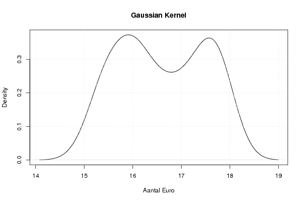
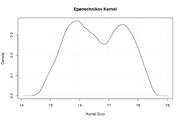
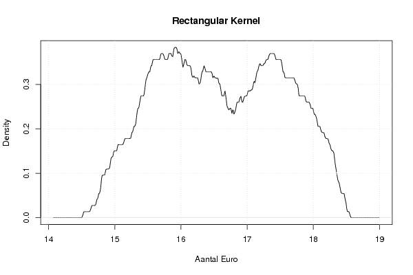
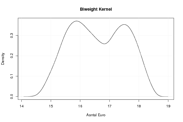
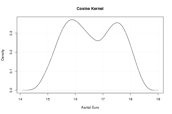
| R Software Module | rwasp_density.wasp | ||||||||||||||||||||||||||||||||
| Title produced by software | Kernel Density Estimation | ||||||||||||||||||||||||||||||||
| Date of computation | Tue, 14 Feb 2012 08:12:10 -0500 | ||||||||||||||||||||||||||||||||
| Cite this page as follows | Statistical Computations at FreeStatistics.org, Office for Research Development and Education, URL https://freestatistics.org/blog/index.php?v=date/2012/Feb/14/t1329225170o0j1tz5wcvr5zop.htm/, Retrieved Mon, 29 Apr 2024 14:51:45 +0000 | ||||||||||||||||||||||||||||||||
| Statistical Computations at FreeStatistics.org, Office for Research Development and Education, URL https://freestatistics.org/blog/index.php?pk=162287, Retrieved Mon, 29 Apr 2024 14:51:45 +0000 | |||||||||||||||||||||||||||||||||
| QR Codes: | |||||||||||||||||||||||||||||||||
|
| |||||||||||||||||||||||||||||||||
| Original text written by user: | |||||||||||||||||||||||||||||||||
| IsPrivate? | No (this computation is public) | ||||||||||||||||||||||||||||||||
| User-defined keywords | |||||||||||||||||||||||||||||||||
| Estimated Impact | 82 | ||||||||||||||||||||||||||||||||
Tree of Dependent Computations | |||||||||||||||||||||||||||||||||
| Family? (F = Feedback message, R = changed R code, M = changed R Module, P = changed Parameters, D = changed Data) | |||||||||||||||||||||||||||||||||
| - [Kernel Density Estimation] [Prijs Evolutie pe...] [2012-02-14 13:12:10] [732e4567293b40941604fcb6ea096e93] [Current] | |||||||||||||||||||||||||||||||||
| Feedback Forum | |||||||||||||||||||||||||||||||||
Post a new message | |||||||||||||||||||||||||||||||||
Dataset | |||||||||||||||||||||||||||||||||
| Dataseries X: | |||||||||||||||||||||||||||||||||
15,13 15,25 15,33 15,36 15,4 15,4 15,41 15,47 15,54 15,55 15,59 15,65 15,75 15,86 15,89 15,94 15,93 15,95 15,99 15,99 16,06 16,08 16,07 16,11 16,15 16,18 16,3 16,42 16,49 16,5 16,58 16,64 16,66 16,81 16,91 16,92 16,95 17,11 17,16 17,16 17,27 17,34 17,39 17,43 17,45 17,5 17,56 17,65 17,62 17,7 17,72 17,71 17,74 17,75 17,78 17,8 17,86 17,88 17,89 17,94 | |||||||||||||||||||||||||||||||||
Tables (Output of Computation) | |||||||||||||||||||||||||||||||||
| |||||||||||||||||||||||||||||||||
Figures (Output of Computation) | |||||||||||||||||||||||||||||||||
Input Parameters & R Code | |||||||||||||||||||||||||||||||||
| Parameters (Session): | |||||||||||||||||||||||||||||||||
| par1 = 0 ; | |||||||||||||||||||||||||||||||||
| Parameters (R input): | |||||||||||||||||||||||||||||||||
| par1 = 0 ; | |||||||||||||||||||||||||||||||||
| R code (references can be found in the software module): | |||||||||||||||||||||||||||||||||
if (par1 == '0') bw <- 'nrd0' | |||||||||||||||||||||||||||||||||