Free Statistics
of Irreproducible Research!
Description of Statistical Computation | |||||||||||||||||||||
|---|---|---|---|---|---|---|---|---|---|---|---|---|---|---|---|---|---|---|---|---|---|
| Author's title | |||||||||||||||||||||
| Author | *Unverified author* | ||||||||||||||||||||
| R Software Module | rwasp_meanplot.wasp | ||||||||||||||||||||
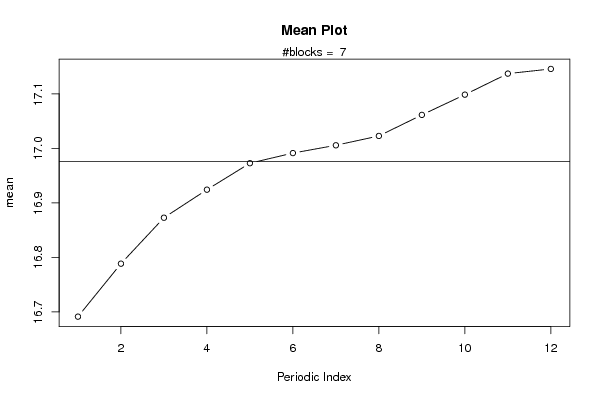
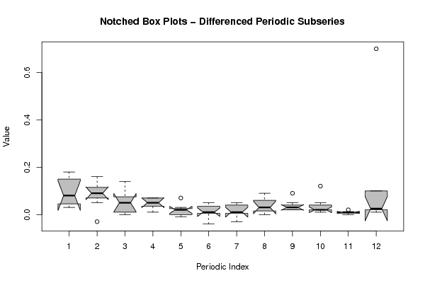
| Title produced by software | Mean Plot | ||||||||||||||||||||
| Date of computation | Wed, 26 Oct 2011 15:18:25 -0400 | ||||||||||||||||||||
| Cite this page as follows | Statistical Computations at FreeStatistics.org, Office for Research Development and Education, URL https://freestatistics.org/blog/index.php?v=date/2011/Oct/26/t1319657035wc867tm1674b2nf.htm/, Retrieved Wed, 15 May 2024 07:14:01 +0000 | ||||||||||||||||||||
| Statistical Computations at FreeStatistics.org, Office for Research Development and Education, URL https://freestatistics.org/blog/index.php?pk=136760, Retrieved Wed, 15 May 2024 07:14:01 +0000 | |||||||||||||||||||||
| QR Codes: | |||||||||||||||||||||
|
| |||||||||||||||||||||
| Original text written by user: | |||||||||||||||||||||
| IsPrivate? | No (this computation is public) | ||||||||||||||||||||
| User-defined keywords | KDG201162 | ||||||||||||||||||||
| Estimated Impact | 85 | ||||||||||||||||||||
Tree of Dependent Computations | |||||||||||||||||||||
| Family? (F = Feedback message, R = changed R code, M = changed R Module, P = changed Parameters, D = changed Data) | |||||||||||||||||||||
| - [Mean Plot] [] [2011-10-26 19:18:25] [df3d6db53fdf346bf57a43ea3fa80561] [Current] | |||||||||||||||||||||
| Feedback Forum | |||||||||||||||||||||
Post a new message | |||||||||||||||||||||
Dataset | |||||||||||||||||||||
| Dataseries X: | |||||||||||||||||||||
14,66 14,71 14,87 14,94 15,01 15,03 15,04 15,05 15,06 15,11 15,23 15,23 15,25 15,33 15,38 15,52 15,59 15,66 15,67 15,72 15,75 15,77 15,79 15,79 16,49 16,67 16,64 16,66 16,73 16,76 16,76 16,76 16,76 16,79 16,8 16,81 16,91 17,03 17,12 17,2 17,25 17,25 17,3 17,27 17,31 17,33 17,35 17,36 17,39 17,42 17,54 17,59 17,64 17,63 17,67 17,7 17,78 17,87 17,9 17,91 17,93 17,97 18,08 18,08 18,09 18,09 18,12 18,13 18,15 18,17 18,19 18,2 18,21 18,39 18,48 18,48 18,5 18,52 18,48 18,53 18,62 18,65 18,7 18,72 | |||||||||||||||||||||
Tables (Output of Computation) | |||||||||||||||||||||
| |||||||||||||||||||||
Figures (Output of Computation) | |||||||||||||||||||||
Input Parameters & R Code | |||||||||||||||||||||
| Parameters (Session): | |||||||||||||||||||||
| par1 = 12 ; | |||||||||||||||||||||
| Parameters (R input): | |||||||||||||||||||||
| par1 = 12 ; | |||||||||||||||||||||
| R code (references can be found in the software module): | |||||||||||||||||||||
par1 <- as.numeric(par1) | |||||||||||||||||||||