\begin{tabular}{lllllllll}
\hline
Summary of computational transaction \tabularnewline
Raw Input & view raw input (R code)  \tabularnewline
Raw Output & view raw output of R engine  \tabularnewline
Computing time & 0 seconds \tabularnewline
R Server & 'Gwilym Jenkins' @ jenkins.wessa.net \tabularnewline
\hline
\end{tabular}
%Source: https://freestatistics.org/blog/index.php?pk=126789&T=0
[TABLE]
[ROW][C]Summary of computational transaction[/C][/ROW]
[ROW][C]Raw Input[/C][C]view raw input (R code) [/C][/ROW]
[ROW][C]Raw Output[/C][C]view raw output of R engine [/C][/ROW]
[ROW][C]Computing time[/C][C]0 seconds[/C][/ROW]
[ROW][C]R Server[/C][C]'Gwilym Jenkins' @ jenkins.wessa.net[/C][/ROW]
[/TABLE]
Source: https://freestatistics.org/blog/index.php?pk=126789&T=0
If you paste this QR Code into your document, anyone with a smartphone or tablet will be able to scan it and view this table in a browser.
If you paste this QR Code into your document, anyone with a smartphone or tablet will be able to scan it and view this table in a browser.
If you paste this QR Code into your document, anyone with a smartphone or tablet will be able to scan it and view this table in a browser.
If you paste this QR Code into your document, anyone with a smartphone or tablet will be able to scan it and view this table in a browser.
If you paste this QR Code into your document, anyone with a smartphone or tablet will be able to scan it and view this table in a browser.
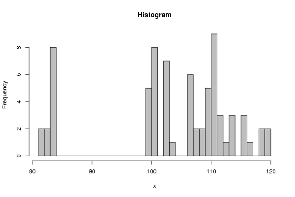
| Frequency Table (Histogram) | | Bins | Midpoint | Abs. Frequency | Rel. Frequency | Cumul. Rel. Freq. | Density | | [81,82[ | 81.5 | 2 | 0.027778 | 0.027778 | 0.027778 | | [82,83[ | 82.5 | 2 | 0.027778 | 0.055556 | 0.027778 | | [83,84[ | 83.5 | 8 | 0.111111 | 0.166667 | 0.111111 | | [84,85[ | 84.5 | 0 | 0 | 0.166667 | 0 | | [85,86[ | 85.5 | 0 | 0 | 0.166667 | 0 | | [86,87[ | 86.5 | 0 | 0 | 0.166667 | 0 | | [87,88[ | 87.5 | 0 | 0 | 0.166667 | 0 | | [88,89[ | 88.5 | 0 | 0 | 0.166667 | 0 | | [89,90[ | 89.5 | 0 | 0 | 0.166667 | 0 | | [90,91[ | 90.5 | 0 | 0 | 0.166667 | 0 | | [91,92[ | 91.5 | 0 | 0 | 0.166667 | 0 | | [92,93[ | 92.5 | 0 | 0 | 0.166667 | 0 | | [93,94[ | 93.5 | 0 | 0 | 0.166667 | 0 | | [94,95[ | 94.5 | 0 | 0 | 0.166667 | 0 | | [95,96[ | 95.5 | 0 | 0 | 0.166667 | 0 | | [96,97[ | 96.5 | 0 | 0 | 0.166667 | 0 | | [97,98[ | 97.5 | 0 | 0 | 0.166667 | 0 | | [98,99[ | 98.5 | 0 | 0 | 0.166667 | 0 | | [99,100[ | 99.5 | 5 | 0.069444 | 0.236111 | 0.069444 | | [100,101[ | 100.5 | 8 | 0.111111 | 0.347222 | 0.111111 | | [101,102[ | 101.5 | 0 | 0 | 0.347222 | 0 | | [102,103[ | 102.5 | 7 | 0.097222 | 0.444444 | 0.097222 | | [103,104[ | 103.5 | 1 | 0.013889 | 0.458333 | 0.013889 | | [104,105[ | 104.5 | 0 | 0 | 0.458333 | 0 | | [105,106[ | 105.5 | 0 | 0 | 0.458333 | 0 | | [106,107[ | 106.5 | 6 | 0.083333 | 0.541667 | 0.083333 | | [107,108[ | 107.5 | 2 | 0.027778 | 0.569444 | 0.027778 | | [108,109[ | 108.5 | 2 | 0.027778 | 0.597222 | 0.027778 | | [109,110[ | 109.5 | 5 | 0.069444 | 0.666667 | 0.069444 | | [110,111[ | 110.5 | 9 | 0.125 | 0.791667 | 0.125 | | [111,112[ | 111.5 | 3 | 0.041667 | 0.833333 | 0.041667 | | [112,113[ | 112.5 | 1 | 0.013889 | 0.847222 | 0.013889 | | [113,114[ | 113.5 | 3 | 0.041667 | 0.888889 | 0.041667 | | [114,115[ | 114.5 | 0 | 0 | 0.888889 | 0 | | [115,116[ | 115.5 | 3 | 0.041667 | 0.930556 | 0.041667 | | [116,117[ | 116.5 | 1 | 0.013889 | 0.944444 | 0.013889 | | [117,118[ | 117.5 | 0 | 0 | 0.944444 | 0 | | [118,119[ | 118.5 | 2 | 0.027778 | 0.972222 | 0.027778 | | [119,120] | 119.5 | 2 | 0.027778 | 1 | 0.027778 |
\begin{tabular}{lllllllll}
\hline
Frequency Table (Histogram) \tabularnewline
Bins & Midpoint & Abs. Frequency & Rel. Frequency & Cumul. Rel. Freq. & Density \tabularnewline
[81,82[ & 81.5 & 2 & 0.027778 & 0.027778 & 0.027778 \tabularnewline
[82,83[ & 82.5 & 2 & 0.027778 & 0.055556 & 0.027778 \tabularnewline
[83,84[ & 83.5 & 8 & 0.111111 & 0.166667 & 0.111111 \tabularnewline
[84,85[ & 84.5 & 0 & 0 & 0.166667 & 0 \tabularnewline
[85,86[ & 85.5 & 0 & 0 & 0.166667 & 0 \tabularnewline
[86,87[ & 86.5 & 0 & 0 & 0.166667 & 0 \tabularnewline
[87,88[ & 87.5 & 0 & 0 & 0.166667 & 0 \tabularnewline
[88,89[ & 88.5 & 0 & 0 & 0.166667 & 0 \tabularnewline
[89,90[ & 89.5 & 0 & 0 & 0.166667 & 0 \tabularnewline
[90,91[ & 90.5 & 0 & 0 & 0.166667 & 0 \tabularnewline
[91,92[ & 91.5 & 0 & 0 & 0.166667 & 0 \tabularnewline
[92,93[ & 92.5 & 0 & 0 & 0.166667 & 0 \tabularnewline
[93,94[ & 93.5 & 0 & 0 & 0.166667 & 0 \tabularnewline
[94,95[ & 94.5 & 0 & 0 & 0.166667 & 0 \tabularnewline
[95,96[ & 95.5 & 0 & 0 & 0.166667 & 0 \tabularnewline
[96,97[ & 96.5 & 0 & 0 & 0.166667 & 0 \tabularnewline
[97,98[ & 97.5 & 0 & 0 & 0.166667 & 0 \tabularnewline
[98,99[ & 98.5 & 0 & 0 & 0.166667 & 0 \tabularnewline
[99,100[ & 99.5 & 5 & 0.069444 & 0.236111 & 0.069444 \tabularnewline
[100,101[ & 100.5 & 8 & 0.111111 & 0.347222 & 0.111111 \tabularnewline
[101,102[ & 101.5 & 0 & 0 & 0.347222 & 0 \tabularnewline
[102,103[ & 102.5 & 7 & 0.097222 & 0.444444 & 0.097222 \tabularnewline
[103,104[ & 103.5 & 1 & 0.013889 & 0.458333 & 0.013889 \tabularnewline
[104,105[ & 104.5 & 0 & 0 & 0.458333 & 0 \tabularnewline
[105,106[ & 105.5 & 0 & 0 & 0.458333 & 0 \tabularnewline
[106,107[ & 106.5 & 6 & 0.083333 & 0.541667 & 0.083333 \tabularnewline
[107,108[ & 107.5 & 2 & 0.027778 & 0.569444 & 0.027778 \tabularnewline
[108,109[ & 108.5 & 2 & 0.027778 & 0.597222 & 0.027778 \tabularnewline
[109,110[ & 109.5 & 5 & 0.069444 & 0.666667 & 0.069444 \tabularnewline
[110,111[ & 110.5 & 9 & 0.125 & 0.791667 & 0.125 \tabularnewline
[111,112[ & 111.5 & 3 & 0.041667 & 0.833333 & 0.041667 \tabularnewline
[112,113[ & 112.5 & 1 & 0.013889 & 0.847222 & 0.013889 \tabularnewline
[113,114[ & 113.5 & 3 & 0.041667 & 0.888889 & 0.041667 \tabularnewline
[114,115[ & 114.5 & 0 & 0 & 0.888889 & 0 \tabularnewline
[115,116[ & 115.5 & 3 & 0.041667 & 0.930556 & 0.041667 \tabularnewline
[116,117[ & 116.5 & 1 & 0.013889 & 0.944444 & 0.013889 \tabularnewline
[117,118[ & 117.5 & 0 & 0 & 0.944444 & 0 \tabularnewline
[118,119[ & 118.5 & 2 & 0.027778 & 0.972222 & 0.027778 \tabularnewline
[119,120] & 119.5 & 2 & 0.027778 & 1 & 0.027778 \tabularnewline
\hline
\end{tabular}
%Source: https://freestatistics.org/blog/index.php?pk=126789&T=1
[TABLE]
[ROW][C]Frequency Table (Histogram)[/C][/ROW]
[ROW][C]Bins[/C][C]Midpoint[/C][C]Abs. Frequency[/C][C]Rel. Frequency[/C][C]Cumul. Rel. Freq.[/C][C]Density[/C][/ROW]
[ROW][C][81,82[[/C][C]81.5[/C][C]2[/C][C]0.027778[/C][C]0.027778[/C][C]0.027778[/C][/ROW]
[ROW][C][82,83[[/C][C]82.5[/C][C]2[/C][C]0.027778[/C][C]0.055556[/C][C]0.027778[/C][/ROW]
[ROW][C][83,84[[/C][C]83.5[/C][C]8[/C][C]0.111111[/C][C]0.166667[/C][C]0.111111[/C][/ROW]
[ROW][C][84,85[[/C][C]84.5[/C][C]0[/C][C]0[/C][C]0.166667[/C][C]0[/C][/ROW]
[ROW][C][85,86[[/C][C]85.5[/C][C]0[/C][C]0[/C][C]0.166667[/C][C]0[/C][/ROW]
[ROW][C][86,87[[/C][C]86.5[/C][C]0[/C][C]0[/C][C]0.166667[/C][C]0[/C][/ROW]
[ROW][C][87,88[[/C][C]87.5[/C][C]0[/C][C]0[/C][C]0.166667[/C][C]0[/C][/ROW]
[ROW][C][88,89[[/C][C]88.5[/C][C]0[/C][C]0[/C][C]0.166667[/C][C]0[/C][/ROW]
[ROW][C][89,90[[/C][C]89.5[/C][C]0[/C][C]0[/C][C]0.166667[/C][C]0[/C][/ROW]
[ROW][C][90,91[[/C][C]90.5[/C][C]0[/C][C]0[/C][C]0.166667[/C][C]0[/C][/ROW]
[ROW][C][91,92[[/C][C]91.5[/C][C]0[/C][C]0[/C][C]0.166667[/C][C]0[/C][/ROW]
[ROW][C][92,93[[/C][C]92.5[/C][C]0[/C][C]0[/C][C]0.166667[/C][C]0[/C][/ROW]
[ROW][C][93,94[[/C][C]93.5[/C][C]0[/C][C]0[/C][C]0.166667[/C][C]0[/C][/ROW]
[ROW][C][94,95[[/C][C]94.5[/C][C]0[/C][C]0[/C][C]0.166667[/C][C]0[/C][/ROW]
[ROW][C][95,96[[/C][C]95.5[/C][C]0[/C][C]0[/C][C]0.166667[/C][C]0[/C][/ROW]
[ROW][C][96,97[[/C][C]96.5[/C][C]0[/C][C]0[/C][C]0.166667[/C][C]0[/C][/ROW]
[ROW][C][97,98[[/C][C]97.5[/C][C]0[/C][C]0[/C][C]0.166667[/C][C]0[/C][/ROW]
[ROW][C][98,99[[/C][C]98.5[/C][C]0[/C][C]0[/C][C]0.166667[/C][C]0[/C][/ROW]
[ROW][C][99,100[[/C][C]99.5[/C][C]5[/C][C]0.069444[/C][C]0.236111[/C][C]0.069444[/C][/ROW]
[ROW][C][100,101[[/C][C]100.5[/C][C]8[/C][C]0.111111[/C][C]0.347222[/C][C]0.111111[/C][/ROW]
[ROW][C][101,102[[/C][C]101.5[/C][C]0[/C][C]0[/C][C]0.347222[/C][C]0[/C][/ROW]
[ROW][C][102,103[[/C][C]102.5[/C][C]7[/C][C]0.097222[/C][C]0.444444[/C][C]0.097222[/C][/ROW]
[ROW][C][103,104[[/C][C]103.5[/C][C]1[/C][C]0.013889[/C][C]0.458333[/C][C]0.013889[/C][/ROW]
[ROW][C][104,105[[/C][C]104.5[/C][C]0[/C][C]0[/C][C]0.458333[/C][C]0[/C][/ROW]
[ROW][C][105,106[[/C][C]105.5[/C][C]0[/C][C]0[/C][C]0.458333[/C][C]0[/C][/ROW]
[ROW][C][106,107[[/C][C]106.5[/C][C]6[/C][C]0.083333[/C][C]0.541667[/C][C]0.083333[/C][/ROW]
[ROW][C][107,108[[/C][C]107.5[/C][C]2[/C][C]0.027778[/C][C]0.569444[/C][C]0.027778[/C][/ROW]
[ROW][C][108,109[[/C][C]108.5[/C][C]2[/C][C]0.027778[/C][C]0.597222[/C][C]0.027778[/C][/ROW]
[ROW][C][109,110[[/C][C]109.5[/C][C]5[/C][C]0.069444[/C][C]0.666667[/C][C]0.069444[/C][/ROW]
[ROW][C][110,111[[/C][C]110.5[/C][C]9[/C][C]0.125[/C][C]0.791667[/C][C]0.125[/C][/ROW]
[ROW][C][111,112[[/C][C]111.5[/C][C]3[/C][C]0.041667[/C][C]0.833333[/C][C]0.041667[/C][/ROW]
[ROW][C][112,113[[/C][C]112.5[/C][C]1[/C][C]0.013889[/C][C]0.847222[/C][C]0.013889[/C][/ROW]
[ROW][C][113,114[[/C][C]113.5[/C][C]3[/C][C]0.041667[/C][C]0.888889[/C][C]0.041667[/C][/ROW]
[ROW][C][114,115[[/C][C]114.5[/C][C]0[/C][C]0[/C][C]0.888889[/C][C]0[/C][/ROW]
[ROW][C][115,116[[/C][C]115.5[/C][C]3[/C][C]0.041667[/C][C]0.930556[/C][C]0.041667[/C][/ROW]
[ROW][C][116,117[[/C][C]116.5[/C][C]1[/C][C]0.013889[/C][C]0.944444[/C][C]0.013889[/C][/ROW]
[ROW][C][117,118[[/C][C]117.5[/C][C]0[/C][C]0[/C][C]0.944444[/C][C]0[/C][/ROW]
[ROW][C][118,119[[/C][C]118.5[/C][C]2[/C][C]0.027778[/C][C]0.972222[/C][C]0.027778[/C][/ROW]
[ROW][C][119,120][/C][C]119.5[/C][C]2[/C][C]0.027778[/C][C]1[/C][C]0.027778[/C][/ROW]
[/TABLE]
Source: https://freestatistics.org/blog/index.php?pk=126789&T=1
Globally Unique Identifier (entire table): ba.freestatistics.org/blog/index.php?pk=126789&T=1
As an alternative you can also use a QR Code:
The GUIDs for individual cells are displayed in the table below:
| Frequency Table (Histogram) | | Bins | Midpoint | Abs. Frequency | Rel. Frequency | Cumul. Rel. Freq. | Density | | [81,82[ | 81.5 | 2 | 0.027778 | 0.027778 | 0.027778 | | [82,83[ | 82.5 | 2 | 0.027778 | 0.055556 | 0.027778 | | [83,84[ | 83.5 | 8 | 0.111111 | 0.166667 | 0.111111 | | [84,85[ | 84.5 | 0 | 0 | 0.166667 | 0 | | [85,86[ | 85.5 | 0 | 0 | 0.166667 | 0 | | [86,87[ | 86.5 | 0 | 0 | 0.166667 | 0 | | [87,88[ | 87.5 | 0 | 0 | 0.166667 | 0 | | [88,89[ | 88.5 | 0 | 0 | 0.166667 | 0 | | [89,90[ | 89.5 | 0 | 0 | 0.166667 | 0 | | [90,91[ | 90.5 | 0 | 0 | 0.166667 | 0 | | [91,92[ | 91.5 | 0 | 0 | 0.166667 | 0 | | [92,93[ | 92.5 | 0 | 0 | 0.166667 | 0 | | [93,94[ | 93.5 | 0 | 0 | 0.166667 | 0 | | [94,95[ | 94.5 | 0 | 0 | 0.166667 | 0 | | [95,96[ | 95.5 | 0 | 0 | 0.166667 | 0 | | [96,97[ | 96.5 | 0 | 0 | 0.166667 | 0 | | [97,98[ | 97.5 | 0 | 0 | 0.166667 | 0 | | [98,99[ | 98.5 | 0 | 0 | 0.166667 | 0 | | [99,100[ | 99.5 | 5 | 0.069444 | 0.236111 | 0.069444 | | [100,101[ | 100.5 | 8 | 0.111111 | 0.347222 | 0.111111 | | [101,102[ | 101.5 | 0 | 0 | 0.347222 | 0 | | [102,103[ | 102.5 | 7 | 0.097222 | 0.444444 | 0.097222 | | [103,104[ | 103.5 | 1 | 0.013889 | 0.458333 | 0.013889 | | [104,105[ | 104.5 | 0 | 0 | 0.458333 | 0 | | [105,106[ | 105.5 | 0 | 0 | 0.458333 | 0 | | [106,107[ | 106.5 | 6 | 0.083333 | 0.541667 | 0.083333 | | [107,108[ | 107.5 | 2 | 0.027778 | 0.569444 | 0.027778 | | [108,109[ | 108.5 | 2 | 0.027778 | 0.597222 | 0.027778 | | [109,110[ | 109.5 | 5 | 0.069444 | 0.666667 | 0.069444 | | [110,111[ | 110.5 | 9 | 0.125 | 0.791667 | 0.125 | | [111,112[ | 111.5 | 3 | 0.041667 | 0.833333 | 0.041667 | | [112,113[ | 112.5 | 1 | 0.013889 | 0.847222 | 0.013889 | | [113,114[ | 113.5 | 3 | 0.041667 | 0.888889 | 0.041667 | | [114,115[ | 114.5 | 0 | 0 | 0.888889 | 0 | | [115,116[ | 115.5 | 3 | 0.041667 | 0.930556 | 0.041667 | | [116,117[ | 116.5 | 1 | 0.013889 | 0.944444 | 0.013889 | | [117,118[ | 117.5 | 0 | 0 | 0.944444 | 0 | | [118,119[ | 118.5 | 2 | 0.027778 | 0.972222 | 0.027778 | | [119,120] | 119.5 | 2 | 0.027778 | 1 | 0.027778 |
If you paste this QR Code into your document, anyone with a smartphone or tablet will be able to scan it and view this table in a browser.
If you paste this QR Code into your document, anyone with a smartphone or tablet will be able to scan it and view this table in a browser.
If you paste this QR Code into your document, anyone with a smartphone or tablet will be able to scan it and view this table in a browser.
If you paste this QR Code into your document, anyone with a smartphone or tablet will be able to scan it and view this table in a browser.
If you paste this QR Code into your document, anyone with a smartphone or tablet will be able to scan it and view this table in a browser.
|