Free Statistics

of Irreproducible Research!

Author's title

Author*Unverified author*
R Software Modulerwasp_density.wasp
Title produced by softwareKernel Density Estimation
Date of computationWed, 05 Oct 2011 11:10:41 -0400
Cite this page as followsStatistical Computations at FreeStatistics.org, Office for Research Development and Education, URL https://freestatistics.org/blog/index.php?v=date/2011/Oct/05/t1317827502pz7sf8bz58655jt.htm/, Retrieved Wed, 15 May 2024 16:09:37 +0000
Statistical Computations at FreeStatistics.org, Office for Research Development and Education, URL https://freestatistics.org/blog/index.php?pk=126723, Retrieved Wed, 15 May 2024 16:09:37 +0000
QR Codes:

Original text written by user:
IsPrivate?No (this computation is public)
User-defined keywordsKDG2011W2EC
Estimated Impact102
Family? (F = Feedback message, R = changed R code, M = changed R Module, P = changed Parameters, D = changed Data)
-       [Kernel Density Estimation] [gemiddelde consum...] [2011-10-05 15:10:41] [08802a004a000ae20ac4145e9a22f7e4] [Current]
Feedback Forum

Post a new message
Dataseries X:
15.14
14.2
13.83
14.31
14.04
14.9
14.92
15.36
15.5
15.65
16.18
15.44
15.58
15.24
15.33
16.07
15.82
15.87
15.72
17.07
16.83
17.52
17.76
17.36
17.95
16.71
17.14
16.72
17.26
17.24
17.69
18.13
18.08
18.18
18.18
17.64
17.89
16.82
16.61
16.66
17.02
16.91
17.18
18.06
17.58
17.48
17.54
17.44
17.79
16.79
16.19
16.62
16.39
16.54
17.26
18
17.29
18.16
17.82
17.48
18.31
17.04
17.03
16.97
17.11
17.12
17.69
18.5
18.27
18.45
18.35
18.03
18.49
18.07
17.8
17.88
18.12
18.68
18.8
19.64
19.56
19.3
20.07
19.82
20.29
19.36
18.74
18.87
18.87
18.91
19.31
20.06
20.72
20.42
20.58
20.58
21.18
19.87
19.83
19.48
19.49
19.4
19.89
20.44
20.07
19.75
19.54
19.07
19.55
18.01
17.5
17.41
17.47
17.6
17.64
18.3
18.27
17.99
18.04
17.62
18.22
17.67
17.73
17.99
18.15
18.41
18.36
19.52
19.96
19.6
19.48
19.13


Summary of computational transaction
Raw Inputview raw input (R code)
Raw Outputview raw output of R engine
Computing time3 seconds
R Server'AstonUniversity' @ aston.wessa.net

\begin{tabular}{lllllllll}
\hline
Summary of computational transaction \tabularnewline
Raw Input & view raw input (R code)  \tabularnewline
Raw Output & view raw output of R engine  \tabularnewline
Computing time & 3 seconds \tabularnewline
R Server & 'AstonUniversity' @ aston.wessa.net \tabularnewline
\hline
\end{tabular}
%Source: https://freestatistics.org/blog/index.php?pk=126723&T=0

[TABLE]
[ROW][C]Summary of computational transaction[/C][/ROW]
[ROW][C]Raw Input[/C][C]view raw input (R code) [/C][/ROW]
[ROW][C]Raw Output[/C][C]view raw output of R engine [/C][/ROW]
[ROW][C]Computing time[/C][C]3 seconds[/C][/ROW]
[ROW][C]R Server[/C][C]'AstonUniversity' @ aston.wessa.net[/C][/ROW]
[/TABLE]
Source: https://freestatistics.org/blog/index.php?pk=126723&T=0

Globally Unique Identifier (entire table): ba.freestatistics.org/blog/index.php?pk=126723&T=0

As an alternative you can also use a QR Code:  

The GUIDs for individual cells are displayed in the table below:

Summary of computational transaction
Raw Inputview raw input (R code)
Raw Outputview raw output of R engine
Computing time3 seconds
R Server'AstonUniversity' @ aston.wessa.net


Properties of Density Trace
Bandwidth0.46604775616965
#Observations132

\begin{tabular}{lllllllll}
\hline
Properties of Density Trace \tabularnewline
Bandwidth & 0.46604775616965 \tabularnewline
#Observations & 132 \tabularnewline
\hline
\end{tabular}
%Source: https://freestatistics.org/blog/index.php?pk=126723&T=1

[TABLE]
[ROW][C]Properties of Density Trace[/C][/ROW]
[ROW][C]Bandwidth[/C][C]0.46604775616965[/C][/ROW]
[ROW][C]#Observations[/C][C]132[/C][/ROW]
[/TABLE]
Source: https://freestatistics.org/blog/index.php?pk=126723&T=1

Globally Unique Identifier (entire table): ba.freestatistics.org/blog/index.php?pk=126723&T=1

As an alternative you can also use a QR Code:  

The GUIDs for individual cells are displayed in the table below:

Properties of Density Trace
Bandwidth0.46604775616965
#Observations132


Parameters (Session):
par1 = 0 ;
Parameters (R input):
par1 = 0 ;
R code (references can be found in the software module):
if (par1 == '0') bw <- 'nrd0'
if (par1 != '0') bw <- as.numeric(par1)
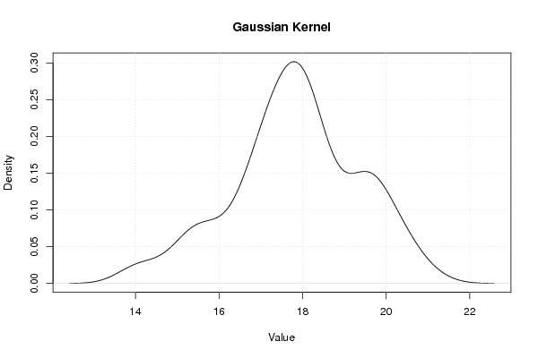
bitmap(file='density1.png')
mydensity1<-density(x,bw=bw,kernel='gaussian',na.rm=TRUE)
plot(mydensity1,main='Gaussian Kernel',xlab=xlab,ylab=ylab)
grid()
dev.off()
mydensity1
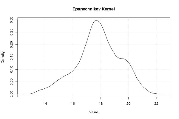
bitmap(file='density2.png')
mydensity2<-density(x,bw=bw,kernel='epanechnikov',na.rm=TRUE)
plot(mydensity2,main='Epanechnikov Kernel',xlab=xlab,ylab=ylab)
grid()
dev.off()
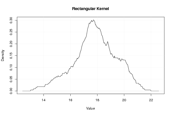
bitmap(file='density3.png')
mydensity3<-density(x,bw=bw,kernel='rectangular',na.rm=TRUE)
plot(mydensity3,main='Rectangular Kernel',xlab=xlab,ylab=ylab)
grid()
dev.off()
bitmap(file='density4.png')
mydensity4<-density(x,bw=bw,kernel='triangular',na.rm=TRUE)
plot(mydensity4,main='Triangular Kernel',xlab=xlab,ylab=ylab)
grid()
dev.off()
bitmap(file='density5.png')
mydensity5<-density(x,bw=bw,kernel='biweight',na.rm=TRUE)
plot(mydensity5,main='Biweight Kernel',xlab=xlab,ylab=ylab)
grid()
dev.off()
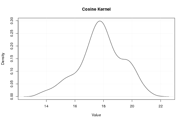
bitmap(file='density6.png')
mydensity6<-density(x,bw=bw,kernel='cosine',na.rm=TRUE)
plot(mydensity6,main='Cosine Kernel',xlab=xlab,ylab=ylab)
grid()
dev.off()
bitmap(file='density7.png')
mydensity7<-density(x,bw=bw,kernel='optcosine',na.rm=TRUE)
plot(mydensity7,main='Optcosine Kernel',xlab=xlab,ylab=ylab)
grid()
dev.off()
load(file='createtable')
a<-table.start()
a<-table.row.start(a)
a<-table.element(a,'Properties of Density Trace',2,TRUE)
a<-table.row.end(a)
a<-table.row.start(a)
a<-table.element(a,'Bandwidth',header=TRUE)
a<-table.element(a,mydensity1$bw)
a<-table.row.end(a)
a<-table.row.start(a)
a<-table.element(a,'#Observations',header=TRUE)
a<-table.element(a,mydensity1$n)
a<-table.row.end(a)
a<-table.end(a)
table.save(a,file='mytable.tab')