Repository of Reproducible Computations

Free Statistics

of Irreproducible Research!

Author's title

Author

*Unverified author*

R Software Module

rwasp_histogram.wasp

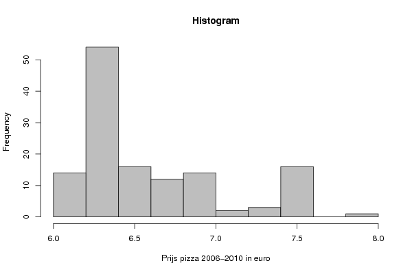
Title produced by software

Histogram

Date of computation

Tue, 04 Oct 2011 11:20:54 -0400

Cite this page as follows

Statistical Computations at FreeStatistics.org, Office for Research Development and Education, URL https://freestatistics.org/blog/index.php?v=date/2011/Oct/04/t1317741708ta7umgmp6h09086.htm/, Retrieved Thu, 16 May 2024 16:55:20 +0000

Statistical Computations at FreeStatistics.org, Office for Research Development and Education, URL https://freestatistics.org/blog/index.php?pk=126083, Retrieved Thu, 16 May 2024 16:55:20 +0000

QR Codes:

Paste this QR Code to cite your computation.

Original text written by user:

IsPrivate?

No (this computation is public)

User-defined keywords

KDGP1W1

Estimated Impact

Family? (F = Feedback message, R = changed R code, M = changed R Module, P = changed Parameters, D = changed Data)

-       [Histogram] [Gemiddelde consum...] [2011-10-04 15:20:54] [ba82c27af75bb26243060ecfbd0283aa] [Current]

Feedback Forum

Post a new message

Dataseries X:

Download CSV

Histogram

Boxplots

6,22
6,19
6,22
6,21
6,21
6,18
6,16
6,18
6,2
6,21
6,18
6,2
6,22
6,27
6,19
6,2
6,28
6,25
6,38
6,36
6,44
6,41
6,38
6,39
6,37
6,33
6,32
6,32
6,3
6,32
6,34
6,38
6,32
6,3
6,32
6,37
6,38
6,38
6,3
6,33
6,26
6,26
6,22
6,21
6,14
6,15
6,17
6,16
6,17
6,18
6,19
6,24
6,28
6,32
6,36
6,39
6,39
6,4
6,4
6,37
6,4
6,39
6,39
6,39
6,39
6,33
6,41
6,45
6,43
6,56
6,57
6,58
6,19
6,31
6,35
6,38
6,38
6,36
6,34
6,49
6,5
6,5
6,55
6,57
6,65
6,61
6,66
6,73
6,73
6,75
6,75
6,71
6,77
6,83
6,9
6,89
7,14
7,35
7,43
7,42
7,41
7,46
7,47
7,45
7,47
7,44
7,43
7,43
7,44
7,49
7,48
7,43
7,33
7,42
7,98
7,41
7,25
7,04
6,98
6,94
6,9
6,92
6,86
6,86
6,89
6,91
6,9
6,88
6,78
6,79
6,81
6,78

Summary of computational transaction
Raw Input	view raw input (R code)
Raw Output	view raw output of R engine
Computing time	0 seconds
R Server	'Gertrude Mary Cox' @ cox.wessa.net

\begin{tabular}{lllllllll}
\hline
Summary of computational transaction \tabularnewline
Raw Input & view raw input (R code)  \tabularnewline
Raw Output & view raw output of R engine  \tabularnewline
Computing time & 0 seconds \tabularnewline
R Server & 'Gertrude Mary Cox' @ cox.wessa.net \tabularnewline
\hline
\end{tabular}
%Source: https://freestatistics.org/blog/index.php?pk=126083&T=0

[TABLE]
[ROW][C]Summary of computational transaction[/C][/ROW]
[ROW][C]Raw Input[/C][C]view raw input (R code) [/C][/ROW]
[ROW][C]Raw Output[/C][C]view raw output of R engine [/C][/ROW]
[ROW][C]Computing time[/C][C]0 seconds[/C][/ROW]
[ROW][C]R Server[/C][C]'Gertrude Mary Cox' @ cox.wessa.net[/C][/ROW]
[/TABLE]
Source: https://freestatistics.org/blog/index.php?pk=126083&T=0

Globally Unique Identifier (entire table): ba.freestatistics.org/blog/index.php?pk=126083&T=0

As an alternative you can also use a QR Code:

The GUIDs for individual cells are displayed in the table below:

Summary of computational transaction
Raw Input	view raw input (R code)
Raw Output	view raw output of R engine
Computing time	0 seconds
R Server	'Gertrude Mary Cox' @ cox.wessa.net

Frequency Table (Histogram)
Bins	Midpoint	Abs. Frequency	Rel. Frequency	Cumul. Rel. Freq.	Density
[6,6.2[	6.1	14	0.106061	0.106061	0.530303
[6.2,6.4[	6.3	54	0.409091	0.515152	2.045455
[6.4,6.6[	6.5	16	0.121212	0.636364	0.606061
[6.6,6.8[	6.7	12	0.090909	0.727273	0.454545
[6.8,7[	6.9	14	0.106061	0.833333	0.530303
[7,7.2[	7.1	2	0.015152	0.848485	0.075758
[7.2,7.4[	7.3	3	0.022727	0.871212	0.113636
[7.4,7.6[	7.5	16	0.121212	0.992424	0.606061
[7.6,7.8[	7.7	0	0	0.992424	0
[7.8,8]	7.9	1	0.007576	1	0.037879

\begin{tabular}{lllllllll}
\hline
Frequency Table (Histogram) \tabularnewline
Bins & Midpoint & Abs. Frequency & Rel. Frequency & Cumul. Rel. Freq. & Density \tabularnewline
[6,6.2[ & 6.1 & 14 & 0.106061 & 0.106061 & 0.530303 \tabularnewline
[6.2,6.4[ & 6.3 & 54 & 0.409091 & 0.515152 & 2.045455 \tabularnewline
[6.4,6.6[ & 6.5 & 16 & 0.121212 & 0.636364 & 0.606061 \tabularnewline
[6.6,6.8[ & 6.7 & 12 & 0.090909 & 0.727273 & 0.454545 \tabularnewline
[6.8,7[ & 6.9 & 14 & 0.106061 & 0.833333 & 0.530303 \tabularnewline
[7,7.2[ & 7.1 & 2 & 0.015152 & 0.848485 & 0.075758 \tabularnewline
[7.2,7.4[ & 7.3 & 3 & 0.022727 & 0.871212 & 0.113636 \tabularnewline
[7.4,7.6[ & 7.5 & 16 & 0.121212 & 0.992424 & 0.606061 \tabularnewline
[7.6,7.8[ & 7.7 & 0 & 0 & 0.992424 & 0 \tabularnewline
[7.8,8] & 7.9 & 1 & 0.007576 & 1 & 0.037879 \tabularnewline
\hline
\end{tabular}
%Source: https://freestatistics.org/blog/index.php?pk=126083&T=1

[TABLE]
[ROW][C]Frequency Table (Histogram)[/C][/ROW]
[ROW][C]Bins[/C][C]Midpoint[/C][C]Abs. Frequency[/C][C]Rel. Frequency[/C][C]Cumul. Rel. Freq.[/C][C]Density[/C][/ROW]
[ROW][C][6,6.2[[/C][C]6.1[/C][C]14[/C][C]0.106061[/C][C]0.106061[/C][C]0.530303[/C][/ROW]
[ROW][C][6.2,6.4[[/C][C]6.3[/C][C]54[/C][C]0.409091[/C][C]0.515152[/C][C]2.045455[/C][/ROW]
[ROW][C][6.4,6.6[[/C][C]6.5[/C][C]16[/C][C]0.121212[/C][C]0.636364[/C][C]0.606061[/C][/ROW]
[ROW][C][6.6,6.8[[/C][C]6.7[/C][C]12[/C][C]0.090909[/C][C]0.727273[/C][C]0.454545[/C][/ROW]
[ROW][C][6.8,7[[/C][C]6.9[/C][C]14[/C][C]0.106061[/C][C]0.833333[/C][C]0.530303[/C][/ROW]
[ROW][C][7,7.2[[/C][C]7.1[/C][C]2[/C][C]0.015152[/C][C]0.848485[/C][C]0.075758[/C][/ROW]
[ROW][C][7.2,7.4[[/C][C]7.3[/C][C]3[/C][C]0.022727[/C][C]0.871212[/C][C]0.113636[/C][/ROW]
[ROW][C][7.4,7.6[[/C][C]7.5[/C][C]16[/C][C]0.121212[/C][C]0.992424[/C][C]0.606061[/C][/ROW]
[ROW][C][7.6,7.8[[/C][C]7.7[/C][C]0[/C][C]0[/C][C]0.992424[/C][C]0[/C][/ROW]
[ROW][C][7.8,8][/C][C]7.9[/C][C]1[/C][C]0.007576[/C][C]1[/C][C]0.037879[/C][/ROW]
[/TABLE]
Source: https://freestatistics.org/blog/index.php?pk=126083&T=1

Globally Unique Identifier (entire table): ba.freestatistics.org/blog/index.php?pk=126083&T=1

As an alternative you can also use a QR Code:

The GUIDs for individual cells are displayed in the table below:

Frequency Table (Histogram)
Bins	Midpoint	Abs. Frequency	Rel. Frequency	Cumul. Rel. Freq.	Density
[6,6.2[	6.1	14	0.106061	0.106061	0.530303
[6.2,6.4[	6.3	54	0.409091	0.515152	2.045455
[6.4,6.6[	6.5	16	0.121212	0.636364	0.606061
[6.6,6.8[	6.7	12	0.090909	0.727273	0.454545
[6.8,7[	6.9	14	0.106061	0.833333	0.530303
[7,7.2[	7.1	2	0.015152	0.848485	0.075758
[7.2,7.4[	7.3	3	0.022727	0.871212	0.113636
[7.4,7.6[	7.5	16	0.121212	0.992424	0.606061
[7.6,7.8[	7.7	0	0	0.992424	0
[7.8,8]	7.9	1	0.007576	1	0.037879

Figure 1

PNG link

Postscript link

PDF link

Parameters (Session):

par1 = 10 ; par2 = grey ; par3 = FALSE ; par4 = Unknown ;

Parameters (R input):

par1 = 10 ; par2 = grey ; par3 = FALSE ; par4 = Unknown ;

R code (references can be found in the software module):

par1 <- as.numeric(par1)
if (par3 == 'TRUE') par3 <- TRUE
if (par3 == 'FALSE') par3 <- FALSE
if (par4 == 'Unknown') par1 <- as.numeric(par1)
if (par4 == 'Interval/Ratio') par1 <- as.numeric(par1)
if (par4 == '3-point Likert') par1 <- c(1:3 - 0.5, 3.5)
if (par4 == '4-point Likert') par1 <- c(1:4 - 0.5, 4.5)
if (par4 == '5-point Likert') par1 <- c(1:5 - 0.5, 5.5)
if (par4 == '6-point Likert') par1 <- c(1:6 - 0.5, 6.5)
if (par4 == '7-point Likert') par1 <- c(1:7 - 0.5, 7.5)
if (par4 == '8-point Likert') par1 <- c(1:8 - 0.5, 8.5)
if (par4 == '9-point Likert') par1 <- c(1:9 - 0.5, 9.5)
if (par4 == '10-point Likert') par1 <- c(1:10 - 0.5, 10.5)
bitmap(file='test1.png')
if(is.numeric(x[1])) {
if (is.na(par1)) {
myhist<-hist(x,col=par2,main=main,xlab=xlab,right=par3)
} else {
if (par1 < 0) par1 <- 3
if (par1 > 50) par1 <- 50
myhist<-hist(x,breaks=par1,col=par2,main=main,xlab=xlab,right=par3)
}
} else {
plot(mytab <- table(x),col=par2,main='Frequency Plot',xlab=xlab,ylab='Absolute Frequency')
}
dev.off()
if(is.numeric(x[1])) {
myhist
n <- length(x)
load(file='createtable')
a<-table.start()
a<-table.row.start(a)
a<-table.element(a,hyperlink('histogram.htm','Frequency Table (Histogram)',''),6,TRUE)
a<-table.row.end(a)
a<-table.row.start(a)
a<-table.element(a,'Bins',header=TRUE)
a<-table.element(a,'Midpoint',header=TRUE)
a<-table.element(a,'Abs. Frequency',header=TRUE)
a<-table.element(a,'Rel. Frequency',header=TRUE)
a<-table.element(a,'Cumul. Rel. Freq.',header=TRUE)
a<-table.element(a,'Density',header=TRUE)
a<-table.row.end(a)
crf <- 0
if (par3 == FALSE) mybracket <- '[' else mybracket <- ']'
mynumrows <- (length(myhist$breaks)-1)
for (i in 1:mynumrows) {
a<-table.row.start(a)
if (i == 1)
dum <- paste('[',myhist$breaks[i],sep='')
else
dum <- paste(mybracket,myhist$breaks[i],sep='')
dum <- paste(dum,myhist$breaks[i+1],sep=',')
if (i==mynumrows)
dum <- paste(dum,']',sep='')
else
dum <- paste(dum,mybracket,sep='')
a<-table.element(a,dum,header=TRUE)
a<-table.element(a,myhist$mids[i])
a<-table.element(a,myhist$counts[i])
rf <- myhist$counts[i]/n
crf <- crf + rf
a<-table.element(a,round(rf,6))
a<-table.element(a,round(crf,6))
a<-table.element(a,round(myhist$density[i],6))
a<-table.row.end(a)
}
a<-table.end(a)
table.save(a,file='mytable.tab')
} else {
mytab
reltab <- mytab / sum(mytab)
n <- length(mytab)
load(file='createtable')
a<-table.start()
a<-table.row.start(a)
a<-table.element(a,'Frequency Table (Categorical Data)',3,TRUE)
a<-table.row.end(a)
a<-table.row.start(a)
a<-table.element(a,'Category',header=TRUE)
a<-table.element(a,'Abs. Frequency',header=TRUE)
a<-table.element(a,'Rel. Frequency',header=TRUE)
a<-table.row.end(a)
for (i in 1:n) {
a<-table.row.start(a)
a<-table.element(a,labels(mytab)$x[i],header=TRUE)
a<-table.element(a,mytab[i])
a<-table.element(a,round(reltab[i],4))
a<-table.row.end(a)
}
a<-table.end(a)
table.save(a,file='mytable1.tab')
}

Free Statistics

Description of Statistical Computation

Tree of Dependent Computations

Dataset

Tables (Output of Computation)

Figures (Output of Computation)

Input Parameters & R Code