Free Statistics
of Irreproducible Research!
Description of Statistical Computation | |||||||||||||||||||||||||||||||||||||||||||||||||||||||||||||||||||||||||||||||||
|---|---|---|---|---|---|---|---|---|---|---|---|---|---|---|---|---|---|---|---|---|---|---|---|---|---|---|---|---|---|---|---|---|---|---|---|---|---|---|---|---|---|---|---|---|---|---|---|---|---|---|---|---|---|---|---|---|---|---|---|---|---|---|---|---|---|---|---|---|---|---|---|---|---|---|---|---|---|---|---|---|---|
| Author's title | |||||||||||||||||||||||||||||||||||||||||||||||||||||||||||||||||||||||||||||||||
| Author | *Unverified author* | ||||||||||||||||||||||||||||||||||||||||||||||||||||||||||||||||||||||||||||||||
| R Software Module | rwasp_bootstrapplot1.wasp | ||||||||||||||||||||||||||||||||||||||||||||||||||||||||||||||||||||||||||||||||
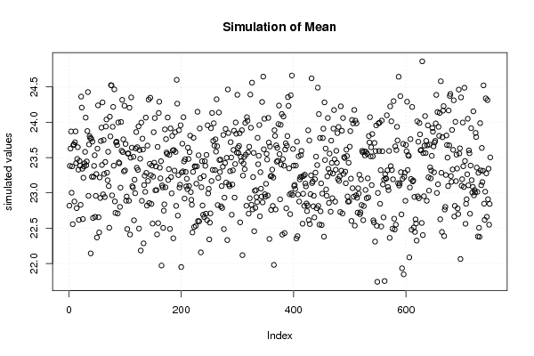
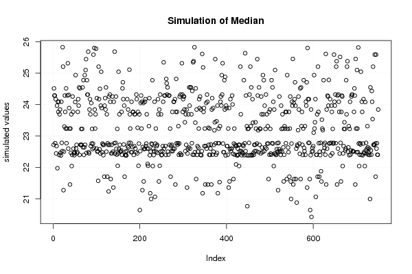
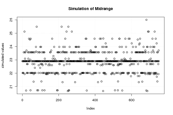
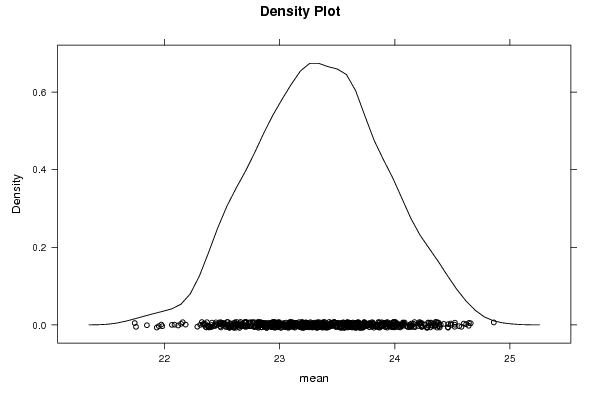
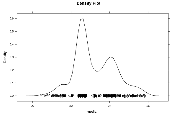
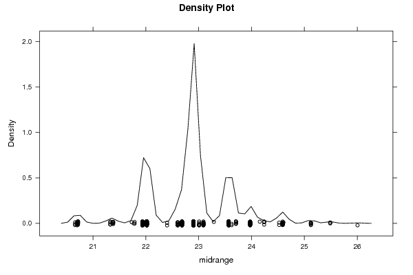
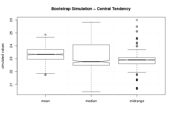
| Title produced by software | Bootstrap Plot - Central Tendency | ||||||||||||||||||||||||||||||||||||||||||||||||||||||||||||||||||||||||||||||||
| Date of computation | Fri, 20 May 2011 03:35:52 +0000 | ||||||||||||||||||||||||||||||||||||||||||||||||||||||||||||||||||||||||||||||||
| Cite this page as follows | Statistical Computations at FreeStatistics.org, Office for Research Development and Education, URL https://freestatistics.org/blog/index.php?v=date/2011/May/20/t130586246763ug028auwg7o8a.htm/, Retrieved Sun, 12 May 2024 19:47:26 +0000 | ||||||||||||||||||||||||||||||||||||||||||||||||||||||||||||||||||||||||||||||||
| Statistical Computations at FreeStatistics.org, Office for Research Development and Education, URL https://freestatistics.org/blog/index.php?pk=122385, Retrieved Sun, 12 May 2024 19:47:26 +0000 | |||||||||||||||||||||||||||||||||||||||||||||||||||||||||||||||||||||||||||||||||
| QR Codes: | |||||||||||||||||||||||||||||||||||||||||||||||||||||||||||||||||||||||||||||||||
|
| |||||||||||||||||||||||||||||||||||||||||||||||||||||||||||||||||||||||||||||||||
| Original text written by user: | |||||||||||||||||||||||||||||||||||||||||||||||||||||||||||||||||||||||||||||||||
| IsPrivate? | No (this computation is public) | ||||||||||||||||||||||||||||||||||||||||||||||||||||||||||||||||||||||||||||||||
| User-defined keywords | KDGP2W22 | ||||||||||||||||||||||||||||||||||||||||||||||||||||||||||||||||||||||||||||||||
| Estimated Impact | 128 | ||||||||||||||||||||||||||||||||||||||||||||||||||||||||||||||||||||||||||||||||
Tree of Dependent Computations | |||||||||||||||||||||||||||||||||||||||||||||||||||||||||||||||||||||||||||||||||
| Family? (F = Feedback message, R = changed R code, M = changed R Module, P = changed Parameters, D = changed Data) | |||||||||||||||||||||||||||||||||||||||||||||||||||||||||||||||||||||||||||||||||
| - [(Partial) Autocorrelation Function] [Autocorrelatie me...] [2009-12-16 11:02:51] [702b109ff2d8b1c8a15cc31390408a4f] - RMPD [Bootstrap Plot - Central Tendency] [Opgave 7: bootstr...] [2011-05-19 20:48:51] [38950998a23e7419c15b25db858fbdfd] - P [Bootstrap Plot - Central Tendency] [Sarah Geerts - bo...] [2011-05-19 22:47:38] [38950998a23e7419c15b25db858fbdfd] - R P [Bootstrap Plot - Central Tendency] [Sarah Geerts - bo...] [2011-05-19 22:51:51] [38950998a23e7419c15b25db858fbdfd] - P [Bootstrap Plot - Central Tendency] [Sarah Geerts - Bo...] [2011-05-20 03:12:40] [38950998a23e7419c15b25db858fbdfd] - R D [Bootstrap Plot - Central Tendency] [Sarah Geerts - Bl...] [2011-05-20 03:35:52] [0b99204a0dc37104849df68eb9128a1a] [Current] | |||||||||||||||||||||||||||||||||||||||||||||||||||||||||||||||||||||||||||||||||
| Feedback Forum | |||||||||||||||||||||||||||||||||||||||||||||||||||||||||||||||||||||||||||||||||
Post a new message | |||||||||||||||||||||||||||||||||||||||||||||||||||||||||||||||||||||||||||||||||
Dataset | |||||||||||||||||||||||||||||||||||||||||||||||||||||||||||||||||||||||||||||||||
| Dataseries X: | |||||||||||||||||||||||||||||||||||||||||||||||||||||||||||||||||||||||||||||||||
31.514 27.071 29.462 26.105 22.397 23.843 21.705 18.089 20.764 25.316 17.704 15.548 28.029 29.383 36.438 32.034 22.679 24.319 18.004 17.537 20.366 22.782 19.169 13.807 29.743 25.591 29.096 26.482 22.405 27.044 17.970 18.730 19.684 19.785 18.479 10.698 31.956 29.506 34.506 27.165 26.736 23.691 18.157 17.328 18.205 20.995 17.382 9.367 31.124 26.551 30.651 25.859 25.100 25.778 20.418 18.688 20.424 24.776 19.814 12.738 31.566 30.111 30.019 31.934 25.826 26.835 20.205 17.789 20.520 22.518 15.572 11.509 25.447 24.090 27.786 26.195 20.516 22.759 19.028 16.971 20.036 22.485 18.730 14.538 27.561 25.985 34.670 32.066 27.186 29.586 21.359 21.553 19.573 24.256 22.380 16.167 27.297 28.287 | |||||||||||||||||||||||||||||||||||||||||||||||||||||||||||||||||||||||||||||||||
Tables (Output of Computation) | |||||||||||||||||||||||||||||||||||||||||||||||||||||||||||||||||||||||||||||||||
| |||||||||||||||||||||||||||||||||||||||||||||||||||||||||||||||||||||||||||||||||
Figures (Output of Computation) | |||||||||||||||||||||||||||||||||||||||||||||||||||||||||||||||||||||||||||||||||
Input Parameters & R Code | |||||||||||||||||||||||||||||||||||||||||||||||||||||||||||||||||||||||||||||||||
| Parameters (Session): | |||||||||||||||||||||||||||||||||||||||||||||||||||||||||||||||||||||||||||||||||
| Parameters (R input): | |||||||||||||||||||||||||||||||||||||||||||||||||||||||||||||||||||||||||||||||||
| par1 = 750 ; | |||||||||||||||||||||||||||||||||||||||||||||||||||||||||||||||||||||||||||||||||
| R code (references can be found in the software module): | |||||||||||||||||||||||||||||||||||||||||||||||||||||||||||||||||||||||||||||||||
par1 <- as.numeric(par1) | |||||||||||||||||||||||||||||||||||||||||||||||||||||||||||||||||||||||||||||||||