Free Statistics
of Irreproducible Research!
Description of Statistical Computation | |||||||||||||||||||||
|---|---|---|---|---|---|---|---|---|---|---|---|---|---|---|---|---|---|---|---|---|---|
| Author's title | |||||||||||||||||||||
| Author | *Unverified author* | ||||||||||||||||||||
| R Software Module | rwasp_sdplot.wasp | ||||||||||||||||||||
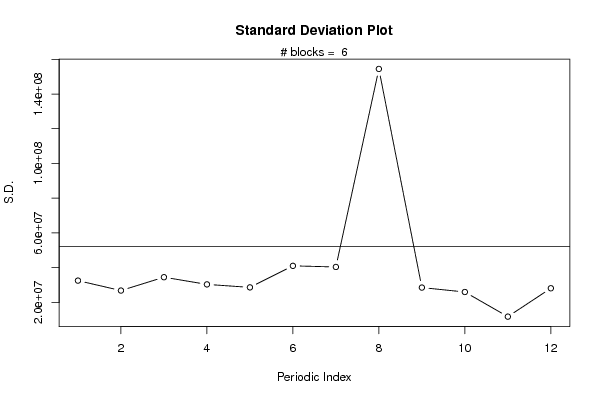
| Title produced by software | Standard Deviation Plot | ||||||||||||||||||||
| Date of computation | Tue, 10 May 2011 17:44:33 +0000 | ||||||||||||||||||||
| Cite this page as follows | Statistical Computations at FreeStatistics.org, Office for Research Development and Education, URL https://freestatistics.org/blog/index.php?v=date/2011/May/10/t1305060468kbo3xowv5pu5nzx.htm/, Retrieved Mon, 13 May 2024 14:22:30 +0000 | ||||||||||||||||||||
| Statistical Computations at FreeStatistics.org, Office for Research Development and Education, URL https://freestatistics.org/blog/index.php?pk=121462, Retrieved Mon, 13 May 2024 14:22:30 +0000 | |||||||||||||||||||||
| QR Codes: | |||||||||||||||||||||
|
| |||||||||||||||||||||
| Original text written by user: | |||||||||||||||||||||
| IsPrivate? | No (this computation is public) | ||||||||||||||||||||
| User-defined keywords | KDGP2W83 | ||||||||||||||||||||
| Estimated Impact | 80 | ||||||||||||||||||||
Tree of Dependent Computations | |||||||||||||||||||||
| Family? (F = Feedback message, R = changed R code, M = changed R Module, P = changed Parameters, D = changed Data) | |||||||||||||||||||||
| - [Standard Deviation Plot] [iko opgave 8 opdr...] [2011-05-10 17:44:33] [93d78dde8d64c5a73537ad1fcc88d508] [Current] - RMP [Classical Decomposition] [IKO opgave 9 oplo...] [2011-05-19 14:12:00] [90e98241b01889302f4a0c1c0db1534e] | |||||||||||||||||||||
| Feedback Forum | |||||||||||||||||||||
Post a new message | |||||||||||||||||||||
Dataset | |||||||||||||||||||||
| Dataseries X: | |||||||||||||||||||||
5939520.00 89948768.00 80953652.00 85942882.00 8944937.00 82975432.00 24940816.00 21973899.00 37950221.00 45949881.00 85950373.00 48960313.00 81954506.00 24960419.00 65973338.00 22950513.00 54963528.00 90995659.00 91967517.00 28999053.00 96990529.00 38979852.00 81496957.00 74982424.00 70976192.00 90990000.00 12998850.00 92986156.00 67994976.00 91022206.00 87992489.00 421022698.00 11018942.00 79100042.00 65996442.00 51000620.00 12996871.00 44994249.00 99996135.00 91977037.00 63974211.00 15998036.00 65974265.00 33984410.00 45939098.00 67935827.00 66921032.00 89911836.00 71890975.00 72880342.00 28871286.00 41844334.00 82847667.00 24871401.00 3867451.00 99896846.00 41890361.00 45884264.00 69884586.00 95896400.00 39904491.00 81900399.00 27909863.00 88900470.00 89917101.00 2945005.00 4934411.00 61957264.00 31946515.00 3938309.00 52933321.00 21947613.00 | |||||||||||||||||||||
Tables (Output of Computation) | |||||||||||||||||||||
| |||||||||||||||||||||
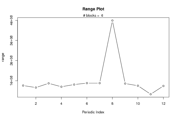
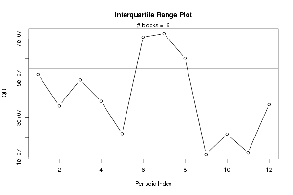
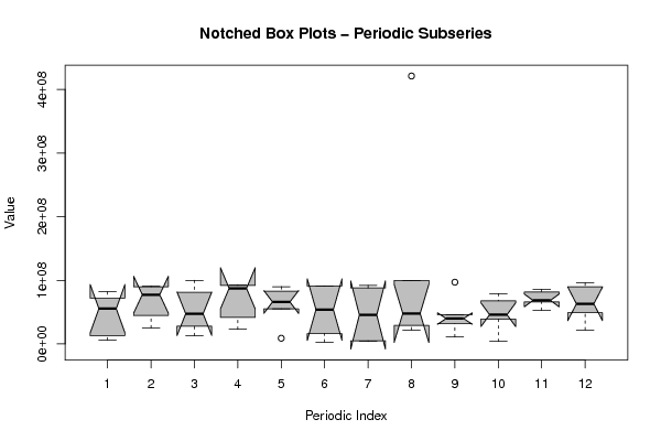
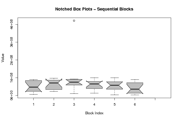
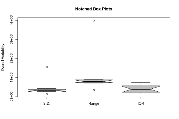
Figures (Output of Computation) | |||||||||||||||||||||
Input Parameters & R Code | |||||||||||||||||||||
| Parameters (Session): | |||||||||||||||||||||
| par1 = 12 ; | |||||||||||||||||||||
| Parameters (R input): | |||||||||||||||||||||
| par1 = 12 ; | |||||||||||||||||||||
| R code (references can be found in the software module): | |||||||||||||||||||||
par1 <- as.numeric(par1) | |||||||||||||||||||||