Free Statistics
of Irreproducible Research!
Description of Statistical Computation | |||||||||||||||||||||
|---|---|---|---|---|---|---|---|---|---|---|---|---|---|---|---|---|---|---|---|---|---|
| Author's title | |||||||||||||||||||||
| Author | *Unverified author* | ||||||||||||||||||||
| R Software Module | rwasp_sdplot.wasp | ||||||||||||||||||||
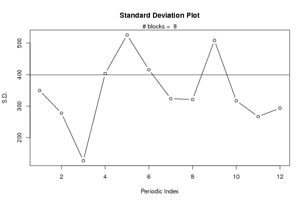
| Title produced by software | Standard Deviation Plot | ||||||||||||||||||||
| Date of computation | Mon, 09 May 2011 20:40:47 +0000 | ||||||||||||||||||||
| Cite this page as follows | Statistical Computations at FreeStatistics.org, Office for Research Development and Education, URL https://freestatistics.org/blog/index.php?v=date/2011/May/09/t1304973552oo79hntv6b61onw.htm/, Retrieved Tue, 14 May 2024 18:47:54 +0000 | ||||||||||||||||||||
| Statistical Computations at FreeStatistics.org, Office for Research Development and Education, URL https://freestatistics.org/blog/index.php?pk=121356, Retrieved Tue, 14 May 2024 18:47:54 +0000 | |||||||||||||||||||||
| QR Codes: | |||||||||||||||||||||
|
| |||||||||||||||||||||
| Original text written by user: | |||||||||||||||||||||
| IsPrivate? | No (this computation is public) | ||||||||||||||||||||
| User-defined keywords | KDGP2W83 | ||||||||||||||||||||
| Estimated Impact | 113 | ||||||||||||||||||||
Tree of Dependent Computations | |||||||||||||||||||||
| Family? (F = Feedback message, R = changed R code, M = changed R Module, P = changed Parameters, D = changed Data) | |||||||||||||||||||||
| - [Variability] [Opdracht 8 IKO - ...] [2011-05-09 08:35:02] [e3e88618d40e1ecdd4fe40f3ead8bcf7] - RMP [Standard Deviation Plot] [Standard Deviatio...] [2011-05-09 20:40:47] [118c7cedabc991c3d34fa0c13010a5e0] [Current] | |||||||||||||||||||||
| Feedback Forum | |||||||||||||||||||||
Post a new message | |||||||||||||||||||||
Dataset | |||||||||||||||||||||
| Dataseries X: | |||||||||||||||||||||
1394 1657 2411 3595 3336 3249 2920 2113 2040 1853 1832 2093 2164 2368 2072 2521 1819 1947 2226 1754 1787 2072 1846 2137 2467 2154 2289 2628 2074 2798 2194 2442 2565 2063 2069 2539 1898 2139 2408 2725 2201 2311 2548 2276 2351 2280 2057 2479 2379 2295 2456 2546 2844 2260 2981 2678 3440 2842 2450 2669 2570 2540 2318 2930 2947 2799 2695 2498 2260 2160 2058 2533 2150 2172 2155 3016 2333 2355 2825 2214 2360 2299 1746 2069 2267 1878 2266 2282 2085 2277 2251 1828 1954 1851 1570 1852 2187 1855 2218 | |||||||||||||||||||||
Tables (Output of Computation) | |||||||||||||||||||||
| |||||||||||||||||||||
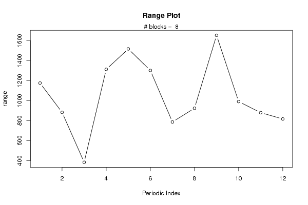
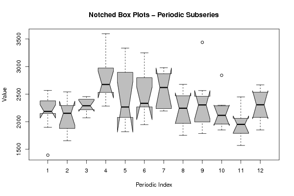
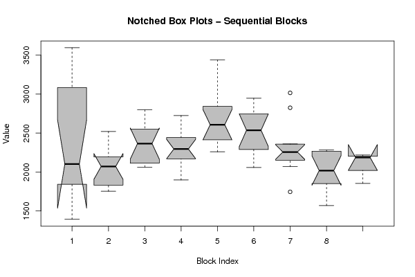
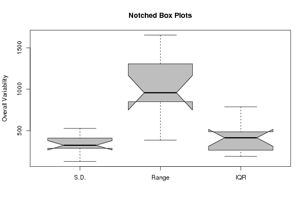
Figures (Output of Computation) | |||||||||||||||||||||
Input Parameters & R Code | |||||||||||||||||||||
| Parameters (Session): | |||||||||||||||||||||
| par1 = 12 ; | |||||||||||||||||||||
| Parameters (R input): | |||||||||||||||||||||
| par1 = 12 ; | |||||||||||||||||||||
| R code (references can be found in the software module): | |||||||||||||||||||||
par1 <- as.numeric(par1) | |||||||||||||||||||||