Free Statistics
of Irreproducible Research!
Description of Statistical Computation | |||||||||||||||||||||
|---|---|---|---|---|---|---|---|---|---|---|---|---|---|---|---|---|---|---|---|---|---|
| Author's title | |||||||||||||||||||||
| Author | *Unverified author* | ||||||||||||||||||||
| R Software Module | rwasp_sdplot.wasp | ||||||||||||||||||||
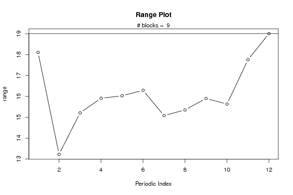
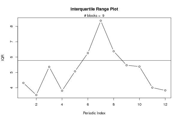
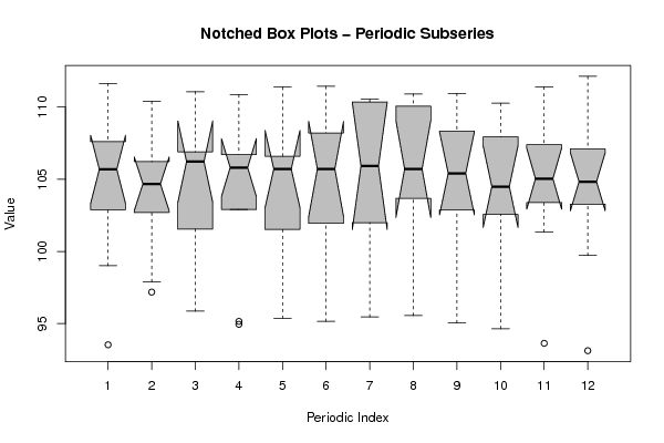
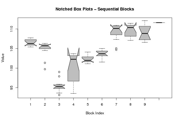
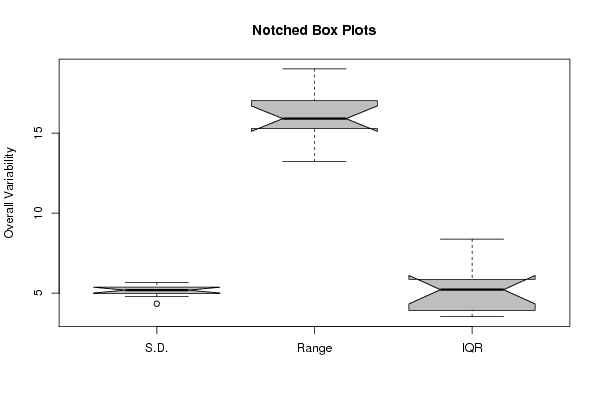
| Title produced by software | Standard Deviation Plot | ||||||||||||||||||||
| Date of computation | Fri, 06 May 2011 12:53:37 +0000 | ||||||||||||||||||||
| Cite this page as follows | Statistical Computations at FreeStatistics.org, Office for Research Development and Education, URL https://freestatistics.org/blog/index.php?v=date/2011/May/06/t1304686245fetqb0qrp896u39.htm/, Retrieved Mon, 13 May 2024 07:21:38 +0000 | ||||||||||||||||||||
| Statistical Computations at FreeStatistics.org, Office for Research Development and Education, URL https://freestatistics.org/blog/index.php?pk=121161, Retrieved Mon, 13 May 2024 07:21:38 +0000 | |||||||||||||||||||||
| QR Codes: | |||||||||||||||||||||
|
| |||||||||||||||||||||
| Original text written by user: | |||||||||||||||||||||
| IsPrivate? | No (this computation is public) | ||||||||||||||||||||
| User-defined keywords | KDGP2W83 | ||||||||||||||||||||
| Estimated Impact | 203 | ||||||||||||||||||||
Tree of Dependent Computations | |||||||||||||||||||||
| Family? (F = Feedback message, R = changed R code, M = changed R Module, P = changed Parameters, D = changed Data) | |||||||||||||||||||||
| - [Standard Deviation Plot] [Isabelle Regnard,...] [2011-05-06 12:53:37] [ed119c57c1c7f005ddf1bbf80b03ea1e] [Current] | |||||||||||||||||||||
| Feedback Forum | |||||||||||||||||||||
Post a new message | |||||||||||||||||||||
Dataset | |||||||||||||||||||||
| Dataseries X: | |||||||||||||||||||||
106,42 106,22 106,32 105,81 105,92 107,54 107,34 107,24 107,74 105,71 105,41 106,22 106,32 106,12 106,22 105,92 105,71 105,71 105,92 105,71 105,41 104,49 101,35 99,72 99,01 97,89 95,86 94,95 95,35 95,15 95,46 95,56 95,05 94,64 93,63 93,12 93,53 97,18 96,27 95,15 97,08 101,95 103,07 103,68 102,87 102,56 103,38 103,27 102,89 102,69 101,54 102,9 101,53 101,96 101,99 101,11 101,75 101,71 104,11 103,57 103,32 103,64 103,68 103,79 103,01 101,54 101,9 103,68 104,62 104,11 105,04 104,83 105,05 104,68 107,32 109,9 109,77 110,69 110,54 110,89 110,95 109,73 110,85 110,39 110,58 110,4 111,07 110,86 111,38 111,44 110,36 110,06 108,34 107,94 107,39 107,1 107,61 107,74 106,9 106,71 106,6 108,21 110,54 110,91 109,51 110,27 111,39 112,13 111,64 | |||||||||||||||||||||
Tables (Output of Computation) | |||||||||||||||||||||
| |||||||||||||||||||||
Figures (Output of Computation) | |||||||||||||||||||||
Input Parameters & R Code | |||||||||||||||||||||
| Parameters (Session): | |||||||||||||||||||||
| par1 = 12 ; | |||||||||||||||||||||
| Parameters (R input): | |||||||||||||||||||||
| par1 = 12 ; | |||||||||||||||||||||
| R code (references can be found in the software module): | |||||||||||||||||||||
par1 <- as.numeric(par1) | |||||||||||||||||||||