Repository of Reproducible Computations

Free Statistics

of Irreproducible Research!

Author's title

Author

*Unverified author*

R Software Module

rwasp_pairs.wasp

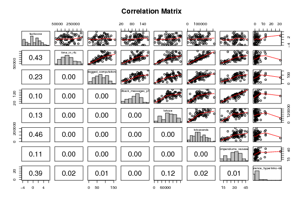
Title produced by software

Kendall tau Correlation Matrix

Date of computation

Mon, 19 Dec 2011 11:21:41 -0500

Cite this page as follows

Statistical Computations at FreeStatistics.org, Office for Research Development and Education, URL https://freestatistics.org/blog/index.php?v=date/2011/Dec/19/t1324311729qs4ax0c79l2k8ux.htm/, Retrieved Wed, 15 May 2024 19:27:18 +0000

Statistical Computations at FreeStatistics.org, Office for Research Development and Education, URL https://freestatistics.org/blog/index.php?pk=157500, Retrieved Wed, 15 May 2024 19:27:18 +0000

QR Codes:

Paste this QR Code to cite your computation.

Original text written by user:

IsPrivate?

No (this computation is public)

User-defined keywords

Estimated Impact

186

Family? (F = Feedback message, R = changed R code, M = changed R Module, P = changed Parameters, D = changed Data)

-     [Kendall tau Correlation Matrix] [paper statistiek,...] [2011-12-19 15:59:25] [4b648d52023f19d55c572f0eddd72b1f]
- R P     [Kendall tau Correlation Matrix] [Paper Kendall Tau] [2011-12-19 16:21:41] [d41d8cd98f00b204e9800998ecf8427e] [Current]
- RMPD      [Multiple Regression] [multiple regressi...] [2011-12-19 17:03:36] [25b6caf3839c2bdc14961e5bff2d6373] 
- RMPD      [Multiple Regression] [Paper Mult. regre...] [2011-12-19 17:48:15] [25b6caf3839c2bdc14961e5bff2d6373] 
-    D        [Multiple Regression] [PAPER - DEEL 3 - ...] [2011-12-21 23:46:47] [da10aa57c5e54f8a2ad733cadd93c4c3] 
- R  D          [Multiple Regression] [PAPER - DEEL 3 - ...] [2011-12-22 13:02:31] [da10aa57c5e54f8a2ad733cadd93c4c3] 
- RMPD          [Recursive Partitioning (Regression Trees)] [PAPER - DEEL 3 - ...] [2011-12-22 16:14:30] [da10aa57c5e54f8a2ad733cadd93c4c3] 
- RMPD          [Recursive Partitioning (Regression Trees)] [PAPER - DEEL 3 - ...] [2011-12-22 16:37:34] [da10aa57c5e54f8a2ad733cadd93c4c3] 
- RMP       [Recursive Partitioning (Regression Trees)] [paper statistiek] [2011-12-19 18:37:20] [4b648d52023f19d55c572f0eddd72b1f] 
-   P         [Recursive Partitioning (Regression Trees)] [paper statistiek] [2011-12-19 22:54:17] [4b648d52023f19d55c572f0eddd72b1f] 
- RMP       [Multiple Regression] [paper statistiek] [2011-12-19 18:47:52] [4b648d52023f19d55c572f0eddd72b1f] 

Feedback Forum

Post a new message

Dataseries X:

Download CSV

Histogram

Boxplots

2	210907	79	94	112285	146283	30	-1
4	179321	108	103	101193	96933	30	3
0	149061	43	93	116174	95757	26	0
0	237213	78	123	66198	143983	38	3
-4	173326	86	148	71701	75851	44	4
4	133131	44	90	57793	59238	30	0
4	258873	104	124	80444	93163	40	0
0	324799	158	168	97668	151511	47	7
-1	230964	102	115	133824	136368	30	1
0	236785	77	71	101481	112642	31	0
1	344297	80	108	67654	127766	30	1
0	174724	123	120	69112	85646	34	4
3	174415	73	114	82753	98579	31	1
-1	223632	105	120	72654	131741	33	5
4	294424	107	124	101494	171975	33	13
3	325107	84	126	79215	159676	36	4
1	106408	33	37	31081	58391	14	0
0	96560	42	38	22996	31580	17	0
-2	265769	96	120	83122	136815	32	6
-3	269651	106	93	70106	120642	30	0
-4	149112	56	95	60578	69107	35	1
2	152871	59	90	79892	108016	28	3
2	362301	76	110	100708	79336	34	1
-4	183167	91	138	82875	93176	39	0
3	277965	115	133	139077	161632	39	2
2	218946	76	96	80670	102996	29	3
2	244052	101	164	143558	160604	44	4
0	341570	94	78	117105	158051	21	12
5	233328	92	102	120733	162647	28	0
-2	206161	75	99	73107	60622	28	3
0	311473	128	129	132068	179566	38	0
-2	207176	56	114	87011	96144	32	4
-3	196553	41	99	95260	129847	29	-1
2	143246	67	104	106671	71180	27	2
2	182192	77	138	70054	86767	40	1
2	194979	66	151	74011	93487	40	1
0	167488	69	72	83737	82981	28	0
4	143756	105	120	69094	73815	34	2
4	275541	116	115	93133	94552	33	0
2	152299	62	98	61370	67808	33	2
2	193339	100	71	84651	106175	35	4
-4	130585	67	107	95364	76669	29	0
3	112611	46	73	26706	57283	20	0
3	148446	135	129	126846	72413	37	6
2	182079	124	118	102860	96971	33	13
-1	243060	58	104	111813	120336	29	4
-3	162765	68	107	120293	93913	28	-1
0	85574	37	36	24266	32036	21	3
1	225060	93	139	109825	102255	41	0
-3	133328	56	56	40909	63506	20	2
3	100750	83	93	140867	68370	30	0
0	101523	59	87	61056	50517	22	1
0	243511	133	110	101338	103950	42	1
0	152474	106	83	65567	84396	32	0
3	132487	71	98	40735	55515	36	31
-3	317394	116	82	91413	209056	31	2
0	244749	98	115	76643	142775	33	5
-4	184510	64	140	110681	68847	40	1
2	128423	32	120	92696	20112	38	1
-1	97839	25	66	94785	61023	24	2
3	172494	46	139	86687	112494	43	13
2	229242	63	119	91721	78876	31	5
5	351619	95	141	115168	170745	40	3
2	324598	113	133	135777	122037	37	1
-2	195838	111	98	102372	112283	31	1
0	254488	120	117	103772	120691	39	4
3	199476	87	105	135400	122422	32	2
-2	92499	25	55	21399	25899	18	0
0	224330	131	132	130115	139296	39	4
6	181633	47	73	64466	89455	30	0
-3	271856	109	86	54990	147866	37	0
3	95227	37	48	34777	14336	32	0
0	98146	15	48	27114	30059	17	7
-2	118612	54	43	30080	41907	12	3
1	65475	16	46	69008	35885	13	4
0	108446	22	65	46300	55764	17	1
2	121848	37	52	30594	35619	17	0
2	76302	29	68	30976	40557	20	2
-3	98104	55	47	25568	44197	17	0
-2	30989	5	41	4154	4103	17	0
1	31774	0	47	4143	4694	17	0
-4	150580	27	71	45588	62991	22	2
0	54157	37	30	18625	24261	15	1
1	59382	29	24	26263	21425	12	0
0	84105	17	63	20055	27184	17	0

Summary of computational transaction
Raw Input	view raw input (R code)
Raw Output	view raw output of R engine
Computing time	2 seconds
R Server	'Gwilym Jenkins' @ jenkins.wessa.net
R Framework error message	The field 'Names of X columns' contains a hard return which cannot be interpreted. Please, resubmit your request without hard returns in the 'Names of X columns'.

\begin{tabular}{lllllllll}
\hline
Summary of computational transaction \tabularnewline
Raw Input & view raw input (R code)  \tabularnewline
Raw Output & view raw output of R engine  \tabularnewline
Computing time & 2 seconds \tabularnewline
R Server & 'Gwilym Jenkins' @ jenkins.wessa.net \tabularnewline
R Framework error message & The field 'Names of X columns' contains a hard return which cannot be interpreted.
Please, resubmit your request without hard returns in the 'Names of X columns'. \tabularnewline
\hline
\end{tabular}
%Source: https://freestatistics.org/blog/index.php?pk=157500&T=0

[TABLE]
[ROW][C]Summary of computational transaction[/C][/ROW]
[ROW][C]Raw Input[/C][C]view raw input (R code) [/C][/ROW]
[ROW][C]Raw Output[/C][C]view raw output of R engine [/C][/ROW]
[ROW][C]Computing time[/C][C]2 seconds[/C][/ROW]
[ROW][C]R Server[/C][C]'Gwilym Jenkins' @ jenkins.wessa.net[/C][/ROW]
[ROW][C]R Framework error message[/C][C]The field 'Names of X columns' contains a hard return which cannot be interpreted.
Please, resubmit your request without hard returns in the 'Names of X columns'.[/C][/ROW]
[/TABLE]
Source: https://freestatistics.org/blog/index.php?pk=157500&T=0

Globally Unique Identifier (entire table): ba.freestatistics.org/blog/index.php?pk=157500&T=0

As an alternative you can also use a QR Code:

The GUIDs for individual cells are displayed in the table below:

Summary of computational transaction
Raw Input	view raw input (R code)
Raw Output	view raw output of R engine
Computing time	2 seconds
R Server	'Gwilym Jenkins' @ jenkins.wessa.net
R Framework error message	The field 'Names of X columns' contains a hard return which cannot be interpreted. Please, resubmit your request without hard returns in the 'Names of X columns'.

Correlations for all pairs of data series (method=kendall)
	testscore	time_in_rfc	blogged_computations	feedback_messages_p120	totsize	totseconds	compendiums_reviewed	difference_hyperlinks-blogs
testscore	1	0.062	0.095	0.127	0.12	0.058	0.125	0.072
time_in_rfc	0.062	1	0.563	0.483	0.469	0.722	0.453	0.185
blogged_computations	0.095	0.563	1	0.467	0.441	0.55	0.508	0.195
feedback_messages_p120	0.127	0.483	0.467	1	0.453	0.444	0.724	0.245
totsize	0.12	0.469	0.441	0.453	1	0.524	0.347	0.124
totseconds	0.058	0.722	0.55	0.444	0.524	1	0.404	0.18
compendiums_reviewed	0.125	0.453	0.508	0.724	0.347	0.404	1	0.208
difference_hyperlinks-blogs	0.072	0.185	0.195	0.245	0.124	0.18	0.208	1

\begin{tabular}{lllllllll}
\hline
Correlations for all pairs of data series (method=kendall) \tabularnewline
  & testscore & time_in_rfc & blogged_computations & feedback_messages_p120 & totsize & totseconds & compendiums_reviewed & difference_hyperlinks-blogs
 \tabularnewline
testscore & 1 & 0.062 & 0.095 & 0.127 & 0.12 & 0.058 & 0.125 & 0.072 \tabularnewline
time_in_rfc & 0.062 & 1 & 0.563 & 0.483 & 0.469 & 0.722 & 0.453 & 0.185 \tabularnewline
blogged_computations & 0.095 & 0.563 & 1 & 0.467 & 0.441 & 0.55 & 0.508 & 0.195 \tabularnewline
feedback_messages_p120 & 0.127 & 0.483 & 0.467 & 1 & 0.453 & 0.444 & 0.724 & 0.245 \tabularnewline
totsize & 0.12 & 0.469 & 0.441 & 0.453 & 1 & 0.524 & 0.347 & 0.124 \tabularnewline
totseconds & 0.058 & 0.722 & 0.55 & 0.444 & 0.524 & 1 & 0.404 & 0.18 \tabularnewline
compendiums_reviewed & 0.125 & 0.453 & 0.508 & 0.724 & 0.347 & 0.404 & 1 & 0.208 \tabularnewline
difference_hyperlinks-blogs
 & 0.072 & 0.185 & 0.195 & 0.245 & 0.124 & 0.18 & 0.208 & 1 \tabularnewline
\hline
\end{tabular}
%Source: https://freestatistics.org/blog/index.php?pk=157500&T=1

[TABLE]
[ROW][C]Correlations for all pairs of data series (method=kendall)[/C][/ROW]
[ROW][C] [/C][C]testscore[/C][C]time_in_rfc[/C][C]blogged_computations[/C][C]feedback_messages_p120[/C][C]totsize[/C][C]totseconds[/C][C]compendiums_reviewed[/C][C]difference_hyperlinks-blogs
[/C][/ROW]
[ROW][C]testscore[/C][C]1[/C][C]0.062[/C][C]0.095[/C][C]0.127[/C][C]0.12[/C][C]0.058[/C][C]0.125[/C][C]0.072[/C][/ROW]
[ROW][C]time_in_rfc[/C][C]0.062[/C][C]1[/C][C]0.563[/C][C]0.483[/C][C]0.469[/C][C]0.722[/C][C]0.453[/C][C]0.185[/C][/ROW]
[ROW][C]blogged_computations[/C][C]0.095[/C][C]0.563[/C][C]1[/C][C]0.467[/C][C]0.441[/C][C]0.55[/C][C]0.508[/C][C]0.195[/C][/ROW]
[ROW][C]feedback_messages_p120[/C][C]0.127[/C][C]0.483[/C][C]0.467[/C][C]1[/C][C]0.453[/C][C]0.444[/C][C]0.724[/C][C]0.245[/C][/ROW]
[ROW][C]totsize[/C][C]0.12[/C][C]0.469[/C][C]0.441[/C][C]0.453[/C][C]1[/C][C]0.524[/C][C]0.347[/C][C]0.124[/C][/ROW]
[ROW][C]totseconds[/C][C]0.058[/C][C]0.722[/C][C]0.55[/C][C]0.444[/C][C]0.524[/C][C]1[/C][C]0.404[/C][C]0.18[/C][/ROW]
[ROW][C]compendiums_reviewed[/C][C]0.125[/C][C]0.453[/C][C]0.508[/C][C]0.724[/C][C]0.347[/C][C]0.404[/C][C]1[/C][C]0.208[/C][/ROW]
[ROW][C]difference_hyperlinks-blogs
[/C][C]0.072[/C][C]0.185[/C][C]0.195[/C][C]0.245[/C][C]0.124[/C][C]0.18[/C][C]0.208[/C][C]1[/C][/ROW]
[/TABLE]
Source: https://freestatistics.org/blog/index.php?pk=157500&T=1

Globally Unique Identifier (entire table): ba.freestatistics.org/blog/index.php?pk=157500&T=1

As an alternative you can also use a QR Code:

The GUIDs for individual cells are displayed in the table below:

Correlations for all pairs of data series (method=kendall)
	testscore	time_in_rfc	blogged_computations	feedback_messages_p120	totsize	totseconds	compendiums_reviewed	difference_hyperlinks-blogs
testscore	1	0.062	0.095	0.127	0.12	0.058	0.125	0.072
time_in_rfc	0.062	1	0.563	0.483	0.469	0.722	0.453	0.185
blogged_computations	0.095	0.563	1	0.467	0.441	0.55	0.508	0.195
feedback_messages_p120	0.127	0.483	0.467	1	0.453	0.444	0.724	0.245
totsize	0.12	0.469	0.441	0.453	1	0.524	0.347	0.124
totseconds	0.058	0.722	0.55	0.444	0.524	1	0.404	0.18
compendiums_reviewed	0.125	0.453	0.508	0.724	0.347	0.404	1	0.208
difference_hyperlinks-blogs	0.072	0.185	0.195	0.245	0.124	0.18	0.208	1

Correlations for all pairs of data series with p-values
pair	Pearson r	Spearman rho	Kendall tau
testscore;time_in_rfc	0.1108	0.0834	0.062
p-value	(0.3129)	(0.4478)	(0.4262)
testscore;blogged_computations	0.1108	0.1264	0.0946
p-value	(0.3125)	(0.2492)	(0.2258)
testscore;feedback_messages_p120	0.1431	0.1838	0.1271
p-value	(0.1914)	(0.0922)	(0.1046)
testscore;totsize	0.1711	0.1658	0.1195
p-value	(0.1175)	(0.1294)	(0.1251)
testscore;totseconds	0.0848	0.0827	0.0578
p-value	(0.4404)	(0.4516)	(0.4581)
testscore;compendiums_reviewed	0.1561	0.1905	0.1253
p-value	(0.1538)	(0.0808)	(0.1143)
testscore;difference_hyperlinks-blogs	0.1705	0.0893	0.0724
p-value	(0.1187)	(0.4163)	(0.3851)
time_in_rfc;blogged_computations	0.7232	0.7488	0.5631
p-value	(0)	(0)	(0)
time_in_rfc;feedback_messages_p120	0.6536	0.6597	0.4831
p-value	(0)	(0)	(0)
time_in_rfc;totsize	0.632	0.6239	0.4689
p-value	(0)	(0)	(0)
time_in_rfc;totseconds	0.8607	0.8872	0.7221
p-value	(0)	(0)	(0)
time_in_rfc;compendiums_reviewed	0.6352	0.6293	0.453
p-value	(0)	(0)	(0)
time_in_rfc;difference_hyperlinks-blogs	0.1313	0.2452	0.1847
p-value	(0.2311)	(0.0237)	(0.0193)
blogged_computations;feedback_messages_p120	0.6796	0.6492	0.4669
p-value	(0)	(0)	(0)
blogged_computations;totsize	0.6564	0.6222	0.4407
p-value	(0)	(0)	(0)
blogged_computations;totseconds	0.7278	0.7418	0.5496
p-value	(0)	(0)	(0)
blogged_computations;compendiums_reviewed	0.7061	0.6775	0.5078
p-value	(0)	(0)	(0)
blogged_computations;difference_hyperlinks-blogs	0.1809	0.2658	0.1947
p-value	(0.0976)	(0.014)	(0.0138)
feedback_messages_p120;totsize	0.7062	0.6348	0.4533
p-value	(0)	(0)	(0)
feedback_messages_p120;totseconds	0.628	0.6089	0.4443
p-value	(0)	(0)	(0)
feedback_messages_p120;compendiums_reviewed	0.8967	0.8685	0.7242
p-value	(0)	(0)	(0)
feedback_messages_p120;difference_hyperlinks-blogs	0.2012	0.3376	0.2454
p-value	(0.0649)	(0.0016)	(0.002)
totsize;totseconds	0.7021	0.6926	0.5238
p-value	(0)	(0)	(0)
totsize;compendiums_reviewed	0.6346	0.5081	0.3473
p-value	(0)	(0)	(0)
totsize;difference_hyperlinks-blogs	0.0535	0.1613	0.1241
p-value	(0.6268)	(0.1402)	(0.116)
totseconds;compendiums_reviewed	0.5953	0.5547	0.4039
p-value	(0)	(0)	(0)
totseconds;difference_hyperlinks-blogs	0.1415	0.2484	0.1798
p-value	(0.1963)	(0.0219)	(0.0227)
compendiums_reviewed;difference_hyperlinks-blogs	0.1961	0.2844	0.2075
p-value	(0.0721)	(0.0083)	(0.0098)

\begin{tabular}{lllllllll}
\hline
Correlations for all pairs of data series with p-values \tabularnewline
pair & Pearson r & Spearman rho & Kendall tau \tabularnewline
testscore;time_in_rfc & 0.1108 & 0.0834 & 0.062 \tabularnewline
p-value & (0.3129) & (0.4478) & (0.4262) \tabularnewline
testscore;blogged_computations & 0.1108 & 0.1264 & 0.0946 \tabularnewline
p-value & (0.3125) & (0.2492) & (0.2258) \tabularnewline
testscore;feedback_messages_p120 & 0.1431 & 0.1838 & 0.1271 \tabularnewline
p-value & (0.1914) & (0.0922) & (0.1046) \tabularnewline
testscore;totsize & 0.1711 & 0.1658 & 0.1195 \tabularnewline
p-value & (0.1175) & (0.1294) & (0.1251) \tabularnewline
testscore;totseconds & 0.0848 & 0.0827 & 0.0578 \tabularnewline
p-value & (0.4404) & (0.4516) & (0.4581) \tabularnewline
testscore;compendiums_reviewed & 0.1561 & 0.1905 & 0.1253 \tabularnewline
p-value & (0.1538) & (0.0808) & (0.1143) \tabularnewline
testscore;difference_hyperlinks-blogs
 & 0.1705 & 0.0893 & 0.0724 \tabularnewline
p-value & (0.1187) & (0.4163) & (0.3851) \tabularnewline
time_in_rfc;blogged_computations & 0.7232 & 0.7488 & 0.5631 \tabularnewline
p-value & (0) & (0) & (0) \tabularnewline
time_in_rfc;feedback_messages_p120 & 0.6536 & 0.6597 & 0.4831 \tabularnewline
p-value & (0) & (0) & (0) \tabularnewline
time_in_rfc;totsize & 0.632 & 0.6239 & 0.4689 \tabularnewline
p-value & (0) & (0) & (0) \tabularnewline
time_in_rfc;totseconds & 0.8607 & 0.8872 & 0.7221 \tabularnewline
p-value & (0) & (0) & (0) \tabularnewline
time_in_rfc;compendiums_reviewed & 0.6352 & 0.6293 & 0.453 \tabularnewline
p-value & (0) & (0) & (0) \tabularnewline
time_in_rfc;difference_hyperlinks-blogs
 & 0.1313 & 0.2452 & 0.1847 \tabularnewline
p-value & (0.2311) & (0.0237) & (0.0193) \tabularnewline
blogged_computations;feedback_messages_p120 & 0.6796 & 0.6492 & 0.4669 \tabularnewline
p-value & (0) & (0) & (0) \tabularnewline
blogged_computations;totsize & 0.6564 & 0.6222 & 0.4407 \tabularnewline
p-value & (0) & (0) & (0) \tabularnewline
blogged_computations;totseconds & 0.7278 & 0.7418 & 0.5496 \tabularnewline
p-value & (0) & (0) & (0) \tabularnewline
blogged_computations;compendiums_reviewed & 0.7061 & 0.6775 & 0.5078 \tabularnewline
p-value & (0) & (0) & (0) \tabularnewline
blogged_computations;difference_hyperlinks-blogs
 & 0.1809 & 0.2658 & 0.1947 \tabularnewline
p-value & (0.0976) & (0.014) & (0.0138) \tabularnewline
feedback_messages_p120;totsize & 0.7062 & 0.6348 & 0.4533 \tabularnewline
p-value & (0) & (0) & (0) \tabularnewline
feedback_messages_p120;totseconds & 0.628 & 0.6089 & 0.4443 \tabularnewline
p-value & (0) & (0) & (0) \tabularnewline
feedback_messages_p120;compendiums_reviewed & 0.8967 & 0.8685 & 0.7242 \tabularnewline
p-value & (0) & (0) & (0) \tabularnewline
feedback_messages_p120;difference_hyperlinks-blogs
 & 0.2012 & 0.3376 & 0.2454 \tabularnewline
p-value & (0.0649) & (0.0016) & (0.002) \tabularnewline
totsize;totseconds & 0.7021 & 0.6926 & 0.5238 \tabularnewline
p-value & (0) & (0) & (0) \tabularnewline
totsize;compendiums_reviewed & 0.6346 & 0.5081 & 0.3473 \tabularnewline
p-value & (0) & (0) & (0) \tabularnewline
totsize;difference_hyperlinks-blogs
 & 0.0535 & 0.1613 & 0.1241 \tabularnewline
p-value & (0.6268) & (0.1402) & (0.116) \tabularnewline
totseconds;compendiums_reviewed & 0.5953 & 0.5547 & 0.4039 \tabularnewline
p-value & (0) & (0) & (0) \tabularnewline
totseconds;difference_hyperlinks-blogs
 & 0.1415 & 0.2484 & 0.1798 \tabularnewline
p-value & (0.1963) & (0.0219) & (0.0227) \tabularnewline
compendiums_reviewed;difference_hyperlinks-blogs
 & 0.1961 & 0.2844 & 0.2075 \tabularnewline
p-value & (0.0721) & (0.0083) & (0.0098) \tabularnewline
\hline
\end{tabular}
%Source: https://freestatistics.org/blog/index.php?pk=157500&T=2

[TABLE]
[ROW][C]Correlations for all pairs of data series with p-values[/C][/ROW]
[ROW][C]pair[/C][C]Pearson r[/C][C]Spearman rho[/C][C]Kendall tau[/C][/ROW]
[ROW][C]testscore;time_in_rfc[/C][C]0.1108[/C][C]0.0834[/C][C]0.062[/C][/ROW]
[ROW][C]p-value[/C][C](0.3129)[/C][C](0.4478)[/C][C](0.4262)[/C][/ROW]
[ROW][C]testscore;blogged_computations[/C][C]0.1108[/C][C]0.1264[/C][C]0.0946[/C][/ROW]
[ROW][C]p-value[/C][C](0.3125)[/C][C](0.2492)[/C][C](0.2258)[/C][/ROW]
[ROW][C]testscore;feedback_messages_p120[/C][C]0.1431[/C][C]0.1838[/C][C]0.1271[/C][/ROW]
[ROW][C]p-value[/C][C](0.1914)[/C][C](0.0922)[/C][C](0.1046)[/C][/ROW]
[ROW][C]testscore;totsize[/C][C]0.1711[/C][C]0.1658[/C][C]0.1195[/C][/ROW]
[ROW][C]p-value[/C][C](0.1175)[/C][C](0.1294)[/C][C](0.1251)[/C][/ROW]
[ROW][C]testscore;totseconds[/C][C]0.0848[/C][C]0.0827[/C][C]0.0578[/C][/ROW]
[ROW][C]p-value[/C][C](0.4404)[/C][C](0.4516)[/C][C](0.4581)[/C][/ROW]
[ROW][C]testscore;compendiums_reviewed[/C][C]0.1561[/C][C]0.1905[/C][C]0.1253[/C][/ROW]
[ROW][C]p-value[/C][C](0.1538)[/C][C](0.0808)[/C][C](0.1143)[/C][/ROW]
[ROW][C]testscore;difference_hyperlinks-blogs
[/C][C]0.1705[/C][C]0.0893[/C][C]0.0724[/C][/ROW]
[ROW][C]p-value[/C][C](0.1187)[/C][C](0.4163)[/C][C](0.3851)[/C][/ROW]
[ROW][C]time_in_rfc;blogged_computations[/C][C]0.7232[/C][C]0.7488[/C][C]0.5631[/C][/ROW]
[ROW][C]p-value[/C][C](0)[/C][C](0)[/C][C](0)[/C][/ROW]
[ROW][C]time_in_rfc;feedback_messages_p120[/C][C]0.6536[/C][C]0.6597[/C][C]0.4831[/C][/ROW]
[ROW][C]p-value[/C][C](0)[/C][C](0)[/C][C](0)[/C][/ROW]
[ROW][C]time_in_rfc;totsize[/C][C]0.632[/C][C]0.6239[/C][C]0.4689[/C][/ROW]
[ROW][C]p-value[/C][C](0)[/C][C](0)[/C][C](0)[/C][/ROW]
[ROW][C]time_in_rfc;totseconds[/C][C]0.8607[/C][C]0.8872[/C][C]0.7221[/C][/ROW]
[ROW][C]p-value[/C][C](0)[/C][C](0)[/C][C](0)[/C][/ROW]
[ROW][C]time_in_rfc;compendiums_reviewed[/C][C]0.6352[/C][C]0.6293[/C][C]0.453[/C][/ROW]
[ROW][C]p-value[/C][C](0)[/C][C](0)[/C][C](0)[/C][/ROW]
[ROW][C]time_in_rfc;difference_hyperlinks-blogs
[/C][C]0.1313[/C][C]0.2452[/C][C]0.1847[/C][/ROW]
[ROW][C]p-value[/C][C](0.2311)[/C][C](0.0237)[/C][C](0.0193)[/C][/ROW]
[ROW][C]blogged_computations;feedback_messages_p120[/C][C]0.6796[/C][C]0.6492[/C][C]0.4669[/C][/ROW]
[ROW][C]p-value[/C][C](0)[/C][C](0)[/C][C](0)[/C][/ROW]
[ROW][C]blogged_computations;totsize[/C][C]0.6564[/C][C]0.6222[/C][C]0.4407[/C][/ROW]
[ROW][C]p-value[/C][C](0)[/C][C](0)[/C][C](0)[/C][/ROW]
[ROW][C]blogged_computations;totseconds[/C][C]0.7278[/C][C]0.7418[/C][C]0.5496[/C][/ROW]
[ROW][C]p-value[/C][C](0)[/C][C](0)[/C][C](0)[/C][/ROW]
[ROW][C]blogged_computations;compendiums_reviewed[/C][C]0.7061[/C][C]0.6775[/C][C]0.5078[/C][/ROW]
[ROW][C]p-value[/C][C](0)[/C][C](0)[/C][C](0)[/C][/ROW]
[ROW][C]blogged_computations;difference_hyperlinks-blogs
[/C][C]0.1809[/C][C]0.2658[/C][C]0.1947[/C][/ROW]
[ROW][C]p-value[/C][C](0.0976)[/C][C](0.014)[/C][C](0.0138)[/C][/ROW]
[ROW][C]feedback_messages_p120;totsize[/C][C]0.7062[/C][C]0.6348[/C][C]0.4533[/C][/ROW]
[ROW][C]p-value[/C][C](0)[/C][C](0)[/C][C](0)[/C][/ROW]
[ROW][C]feedback_messages_p120;totseconds[/C][C]0.628[/C][C]0.6089[/C][C]0.4443[/C][/ROW]
[ROW][C]p-value[/C][C](0)[/C][C](0)[/C][C](0)[/C][/ROW]
[ROW][C]feedback_messages_p120;compendiums_reviewed[/C][C]0.8967[/C][C]0.8685[/C][C]0.7242[/C][/ROW]
[ROW][C]p-value[/C][C](0)[/C][C](0)[/C][C](0)[/C][/ROW]
[ROW][C]feedback_messages_p120;difference_hyperlinks-blogs
[/C][C]0.2012[/C][C]0.3376[/C][C]0.2454[/C][/ROW]
[ROW][C]p-value[/C][C](0.0649)[/C][C](0.0016)[/C][C](0.002)[/C][/ROW]
[ROW][C]totsize;totseconds[/C][C]0.7021[/C][C]0.6926[/C][C]0.5238[/C][/ROW]
[ROW][C]p-value[/C][C](0)[/C][C](0)[/C][C](0)[/C][/ROW]
[ROW][C]totsize;compendiums_reviewed[/C][C]0.6346[/C][C]0.5081[/C][C]0.3473[/C][/ROW]
[ROW][C]p-value[/C][C](0)[/C][C](0)[/C][C](0)[/C][/ROW]
[ROW][C]totsize;difference_hyperlinks-blogs
[/C][C]0.0535[/C][C]0.1613[/C][C]0.1241[/C][/ROW]
[ROW][C]p-value[/C][C](0.6268)[/C][C](0.1402)[/C][C](0.116)[/C][/ROW]
[ROW][C]totseconds;compendiums_reviewed[/C][C]0.5953[/C][C]0.5547[/C][C]0.4039[/C][/ROW]
[ROW][C]p-value[/C][C](0)[/C][C](0)[/C][C](0)[/C][/ROW]
[ROW][C]totseconds;difference_hyperlinks-blogs
[/C][C]0.1415[/C][C]0.2484[/C][C]0.1798[/C][/ROW]
[ROW][C]p-value[/C][C](0.1963)[/C][C](0.0219)[/C][C](0.0227)[/C][/ROW]
[ROW][C]compendiums_reviewed;difference_hyperlinks-blogs
[/C][C]0.1961[/C][C]0.2844[/C][C]0.2075[/C][/ROW]
[ROW][C]p-value[/C][C](0.0721)[/C][C](0.0083)[/C][C](0.0098)[/C][/ROW]
[/TABLE]
Source: https://freestatistics.org/blog/index.php?pk=157500&T=2

Globally Unique Identifier (entire table): ba.freestatistics.org/blog/index.php?pk=157500&T=2

As an alternative you can also use a QR Code:

The GUIDs for individual cells are displayed in the table below:

Correlations for all pairs of data series with p-values
pair	Pearson r	Spearman rho	Kendall tau
testscore;time_in_rfc	0.1108	0.0834	0.062
p-value	(0.3129)	(0.4478)	(0.4262)
testscore;blogged_computations	0.1108	0.1264	0.0946
p-value	(0.3125)	(0.2492)	(0.2258)
testscore;feedback_messages_p120	0.1431	0.1838	0.1271
p-value	(0.1914)	(0.0922)	(0.1046)
testscore;totsize	0.1711	0.1658	0.1195
p-value	(0.1175)	(0.1294)	(0.1251)
testscore;totseconds	0.0848	0.0827	0.0578
p-value	(0.4404)	(0.4516)	(0.4581)
testscore;compendiums_reviewed	0.1561	0.1905	0.1253
p-value	(0.1538)	(0.0808)	(0.1143)
testscore;difference_hyperlinks-blogs	0.1705	0.0893	0.0724
p-value	(0.1187)	(0.4163)	(0.3851)
time_in_rfc;blogged_computations	0.7232	0.7488	0.5631
p-value	(0)	(0)	(0)
time_in_rfc;feedback_messages_p120	0.6536	0.6597	0.4831
p-value	(0)	(0)	(0)
time_in_rfc;totsize	0.632	0.6239	0.4689
p-value	(0)	(0)	(0)
time_in_rfc;totseconds	0.8607	0.8872	0.7221
p-value	(0)	(0)	(0)
time_in_rfc;compendiums_reviewed	0.6352	0.6293	0.453
p-value	(0)	(0)	(0)
time_in_rfc;difference_hyperlinks-blogs	0.1313	0.2452	0.1847
p-value	(0.2311)	(0.0237)	(0.0193)
blogged_computations;feedback_messages_p120	0.6796	0.6492	0.4669
p-value	(0)	(0)	(0)
blogged_computations;totsize	0.6564	0.6222	0.4407
p-value	(0)	(0)	(0)
blogged_computations;totseconds	0.7278	0.7418	0.5496
p-value	(0)	(0)	(0)
blogged_computations;compendiums_reviewed	0.7061	0.6775	0.5078
p-value	(0)	(0)	(0)
blogged_computations;difference_hyperlinks-blogs	0.1809	0.2658	0.1947
p-value	(0.0976)	(0.014)	(0.0138)
feedback_messages_p120;totsize	0.7062	0.6348	0.4533
p-value	(0)	(0)	(0)
feedback_messages_p120;totseconds	0.628	0.6089	0.4443
p-value	(0)	(0)	(0)
feedback_messages_p120;compendiums_reviewed	0.8967	0.8685	0.7242
p-value	(0)	(0)	(0)
feedback_messages_p120;difference_hyperlinks-blogs	0.2012	0.3376	0.2454
p-value	(0.0649)	(0.0016)	(0.002)
totsize;totseconds	0.7021	0.6926	0.5238
p-value	(0)	(0)	(0)
totsize;compendiums_reviewed	0.6346	0.5081	0.3473
p-value	(0)	(0)	(0)
totsize;difference_hyperlinks-blogs	0.0535	0.1613	0.1241
p-value	(0.6268)	(0.1402)	(0.116)
totseconds;compendiums_reviewed	0.5953	0.5547	0.4039
p-value	(0)	(0)	(0)
totseconds;difference_hyperlinks-blogs	0.1415	0.2484	0.1798
p-value	(0.1963)	(0.0219)	(0.0227)
compendiums_reviewed;difference_hyperlinks-blogs	0.1961	0.2844	0.2075
p-value	(0.0721)	(0.0083)	(0.0098)

Figure 1

PNG link

Postscript link

PDF link

Parameters (Session):

par1 = kendall ;

Parameters (R input):

par1 = kendall ;

R code (references can be found in the software module):

panel.tau <- function(x, y, digits=2, prefix='', cex.cor)
{
usr <- par('usr'); on.exit(par(usr))
par(usr = c(0, 1, 0, 1))
rr <- cor.test(x, y, method=par1)
r <- round(rr$p.value,2)
txt <- format(c(r, 0.123456789), digits=digits)[1]
txt <- paste(prefix, txt, sep='')
if(missing(cex.cor)) cex <- 0.5/strwidth(txt)
text(0.5, 0.5, txt, cex = cex)
}
panel.hist <- function(x, ...)
{
usr <- par('usr'); on.exit(par(usr))
par(usr = c(usr[1:2], 0, 1.5) )
h <- hist(x, plot = FALSE)
breaks <- h$breaks; nB <- length(breaks)
y <- h$counts; y <- y/max(y)
rect(breaks[-nB], 0, breaks[-1], y, col='grey', ...)
}
bitmap(file='test1.png')
pairs(t(y),diag.panel=panel.hist, upper.panel=panel.smooth, lower.panel=panel.tau, main=main)
dev.off()
load(file='createtable')
n <- length(y[,1])
n
a<-table.start()
a<-table.row.start(a)
a<-table.element(a,paste('Correlations for all pairs of data series (method=',par1,')',sep=''),n+1,TRUE)
a<-table.row.end(a)
a<-table.row.start(a)
a<-table.element(a,' ',header=TRUE)
for (i in 1:n) {
a<-table.element(a,dimnames(t(x))[[2]][i],header=TRUE)
}
a<-table.row.end(a)
for (i in 1:n) {
a<-table.row.start(a)
a<-table.element(a,dimnames(t(x))[[2]][i],header=TRUE)
for (j in 1:n) {
r <- cor.test(y[i,],y[j,],method=par1)
a<-table.element(a,round(r$estimate,3))
}
a<-table.row.end(a)
}
a<-table.end(a)
table.save(a,file='mytable.tab')
a<-table.start()
a<-table.row.start(a)
a<-table.element(a,'Correlations for all pairs of data series with p-values',4,TRUE)
a<-table.row.end(a)
a<-table.row.start(a)
a<-table.element(a,'pair',1,TRUE)
a<-table.element(a,'Pearson r',1,TRUE)
a<-table.element(a,'Spearman rho',1,TRUE)
a<-table.element(a,'Kendall tau',1,TRUE)
a<-table.row.end(a)
cor.test(y[1,],y[2,],method=par1)
for (i in 1:(n-1))
{
for (j in (i+1):n)
{
a<-table.row.start(a)
dum <- paste(dimnames(t(x))[[2]][i],';',dimnames(t(x))[[2]][j],sep='')
a<-table.element(a,dum,header=TRUE)
rp <- cor.test(y[i,],y[j,],method='pearson')
a<-table.element(a,round(rp$estimate,4))
rs <- cor.test(y[i,],y[j,],method='spearman')
a<-table.element(a,round(rs$estimate,4))
rk <- cor.test(y[i,],y[j,],method='kendall')
a<-table.element(a,round(rk$estimate,4))
a<-table.row.end(a)
a<-table.row.start(a)
a<-table.element(a,'p-value',header=T)
a<-table.element(a,paste('(',round(rp$p.value,4),')',sep=''))
a<-table.element(a,paste('(',round(rs$p.value,4),')',sep=''))
a<-table.element(a,paste('(',round(rk$p.value,4),')',sep=''))
a<-table.row.end(a)
}
}
a<-table.end(a)
table.save(a,file='mytable1.tab')

Free Statistics

Description of Statistical Computation

Tree of Dependent Computations

Dataset

Tables (Output of Computation)

Figures (Output of Computation)

Input Parameters & R Code