Repository of Reproducible Computations

Free Statistics

of Irreproducible Research!

Author's title

Author

*The author of this computation has been verified*

R Software Module

rwasp_autocorrelation.wasp

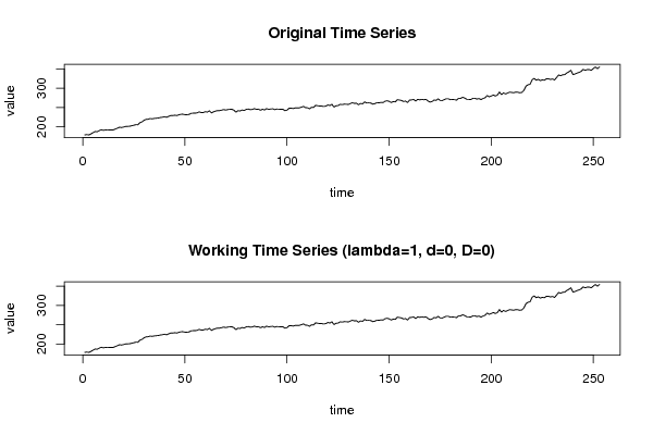
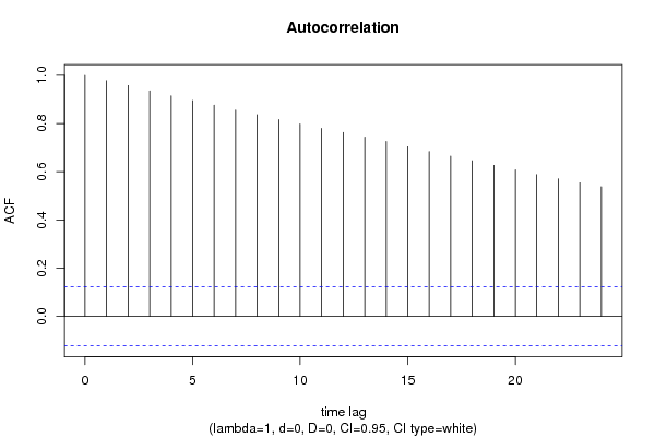
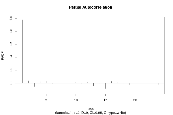
Title produced by software

(Partial) Autocorrelation Function

Date of computation

Mon, 19 Dec 2011 05:10:20 -0500

Cite this page as follows

Statistical Computations at FreeStatistics.org, Office for Research Development and Education, URL https://freestatistics.org/blog/index.php?v=date/2011/Dec/19/t13242897044sg4yhstejikiwr.htm/, Retrieved Wed, 15 May 2024 18:46:46 +0000

Statistical Computations at FreeStatistics.org, Office for Research Development and Education, URL https://freestatistics.org/blog/index.php?pk=157258, Retrieved Wed, 15 May 2024 18:46:46 +0000

QR Codes:

Paste this QR Code to cite your computation.

Original text written by user:

IsPrivate?

No (this computation is public)

User-defined keywords

Estimated Impact

117

Family? (F = Feedback message, R = changed R code, M = changed R Module, P = changed Parameters, D = changed Data)

-     [Univariate Explorative Data Analysis] [Run Sequence gebo...] [2008-12-12 13:32:37] [76963dc1903f0f612b6153510a3818cf]
- R  D  [Univariate Explorative Data Analysis] [Run Sequence gebo...] [2008-12-17 12:14:40] [76963dc1903f0f612b6153510a3818cf]
-         [Univariate Explorative Data Analysis] [Run Sequence Plot...] [2008-12-22 18:19:51] [1ce0d16c8f4225c977b42c8fa93bc163]
- RMP       [Univariate Data Series] [Identifying Integ...] [2009-11-22 12:08:06] [b98453cac15ba1066b407e146608df68]
- RMP         [(Partial) Autocorrelation Function] [Births] [2010-11-29 09:36:27] [b98453cac15ba1066b407e146608df68]
- R PD            [(Partial) Autocorrelation Function] [] [2011-12-19 10:10:20] [c8f7c4812ba63eaa5bf379ee3b4bd6a3] [Current]

Feedback Forum

Post a new message

Dataseries X:

Download CSV

Histogram

Boxplots

Summary of computational transaction
Raw Input	view raw input (R code)
Raw Output	view raw output of R engine
Computing time	1 seconds
R Server	'Gwilym Jenkins' @ jenkins.wessa.net

\begin{tabular}{lllllllll}
\hline
Summary of computational transaction \tabularnewline
Raw Input & view raw input (R code)  \tabularnewline
Raw Output & view raw output of R engine  \tabularnewline
Computing time & 1 seconds \tabularnewline
R Server & 'Gwilym Jenkins' @ jenkins.wessa.net \tabularnewline
\hline
\end{tabular}
%Source: https://freestatistics.org/blog/index.php?pk=157258&T=0

[TABLE]
[ROW][C]Summary of computational transaction[/C][/ROW]
[ROW][C]Raw Input[/C][C]view raw input (R code) [/C][/ROW]
[ROW][C]Raw Output[/C][C]view raw output of R engine [/C][/ROW]
[ROW][C]Computing time[/C][C]1 seconds[/C][/ROW]
[ROW][C]R Server[/C][C]'Gwilym Jenkins' @ jenkins.wessa.net[/C][/ROW]
[/TABLE]
Source: https://freestatistics.org/blog/index.php?pk=157258&T=0

Globally Unique Identifier (entire table): ba.freestatistics.org/blog/index.php?pk=157258&T=0

As an alternative you can also use a QR Code:

The GUIDs for individual cells are displayed in the table below:

Summary of computational transaction
Raw Input	view raw input (R code)
Raw Output	view raw output of R engine
Computing time	1 seconds
R Server	'Gwilym Jenkins' @ jenkins.wessa.net

Autocorrelation Function
Time lag k	ACF(k)	T-STAT	P-value
1	0.977667	15.5507	0
2	0.957366	15.2278	0
3	0.935057	14.873	0
4	0.914407	14.5445	0
5	0.895144	14.2381	0
6	0.876023	13.934	0
7	0.855692	13.6106	0
8	0.836404	13.3038	0
9	0.816531	12.9877	0
10	0.798123	12.6949	0
11	0.779824	12.4039	0
12	0.76254	12.1289	0
13	0.743552	11.8269	0
14	0.725266	11.5361	0
15	0.703422	11.1886	0
16	0.68363	10.8738	0
17	0.664134	10.5637	0
18	0.64555	10.2681	0
19	0.626173	9.9599	0
20	0.60726	9.6591	0
21	0.587704	9.348	0
22	0.570189	9.0694	0
23	0.55367	8.8067	0
24	0.536977	8.5411	0

\begin{tabular}{lllllllll}
\hline
Autocorrelation Function \tabularnewline
Time lag k & ACF(k) & T-STAT & P-value \tabularnewline
1 & 0.977667 & 15.5507 & 0 \tabularnewline
2 & 0.957366 & 15.2278 & 0 \tabularnewline
3 & 0.935057 & 14.873 & 0 \tabularnewline
4 & 0.914407 & 14.5445 & 0 \tabularnewline
5 & 0.895144 & 14.2381 & 0 \tabularnewline
6 & 0.876023 & 13.934 & 0 \tabularnewline
7 & 0.855692 & 13.6106 & 0 \tabularnewline
8 & 0.836404 & 13.3038 & 0 \tabularnewline
9 & 0.816531 & 12.9877 & 0 \tabularnewline
10 & 0.798123 & 12.6949 & 0 \tabularnewline
11 & 0.779824 & 12.4039 & 0 \tabularnewline
12 & 0.76254 & 12.1289 & 0 \tabularnewline
13 & 0.743552 & 11.8269 & 0 \tabularnewline
14 & 0.725266 & 11.5361 & 0 \tabularnewline
15 & 0.703422 & 11.1886 & 0 \tabularnewline
16 & 0.68363 & 10.8738 & 0 \tabularnewline
17 & 0.664134 & 10.5637 & 0 \tabularnewline
18 & 0.64555 & 10.2681 & 0 \tabularnewline
19 & 0.626173 & 9.9599 & 0 \tabularnewline
20 & 0.60726 & 9.6591 & 0 \tabularnewline
21 & 0.587704 & 9.348 & 0 \tabularnewline
22 & 0.570189 & 9.0694 & 0 \tabularnewline
23 & 0.55367 & 8.8067 & 0 \tabularnewline
24 & 0.536977 & 8.5411 & 0 \tabularnewline
\hline
\end{tabular}
%Source: https://freestatistics.org/blog/index.php?pk=157258&T=1

[TABLE]
[ROW][C]Autocorrelation Function[/C][/ROW]
[ROW][C]Time lag k[/C][C]ACF(k)[/C][C]T-STAT[/C][C]P-value[/C][/ROW]
[ROW][C]1[/C][C]0.977667[/C][C]15.5507[/C][C]0[/C][/ROW]
[ROW][C]2[/C][C]0.957366[/C][C]15.2278[/C][C]0[/C][/ROW]
[ROW][C]3[/C][C]0.935057[/C][C]14.873[/C][C]0[/C][/ROW]
[ROW][C]4[/C][C]0.914407[/C][C]14.5445[/C][C]0[/C][/ROW]
[ROW][C]5[/C][C]0.895144[/C][C]14.2381[/C][C]0[/C][/ROW]
[ROW][C]6[/C][C]0.876023[/C][C]13.934[/C][C]0[/C][/ROW]
[ROW][C]7[/C][C]0.855692[/C][C]13.6106[/C][C]0[/C][/ROW]
[ROW][C]8[/C][C]0.836404[/C][C]13.3038[/C][C]0[/C][/ROW]
[ROW][C]9[/C][C]0.816531[/C][C]12.9877[/C][C]0[/C][/ROW]
[ROW][C]10[/C][C]0.798123[/C][C]12.6949[/C][C]0[/C][/ROW]
[ROW][C]11[/C][C]0.779824[/C][C]12.4039[/C][C]0[/C][/ROW]
[ROW][C]12[/C][C]0.76254[/C][C]12.1289[/C][C]0[/C][/ROW]
[ROW][C]13[/C][C]0.743552[/C][C]11.8269[/C][C]0[/C][/ROW]
[ROW][C]14[/C][C]0.725266[/C][C]11.5361[/C][C]0[/C][/ROW]
[ROW][C]15[/C][C]0.703422[/C][C]11.1886[/C][C]0[/C][/ROW]
[ROW][C]16[/C][C]0.68363[/C][C]10.8738[/C][C]0[/C][/ROW]
[ROW][C]17[/C][C]0.664134[/C][C]10.5637[/C][C]0[/C][/ROW]
[ROW][C]18[/C][C]0.64555[/C][C]10.2681[/C][C]0[/C][/ROW]
[ROW][C]19[/C][C]0.626173[/C][C]9.9599[/C][C]0[/C][/ROW]
[ROW][C]20[/C][C]0.60726[/C][C]9.6591[/C][C]0[/C][/ROW]
[ROW][C]21[/C][C]0.587704[/C][C]9.348[/C][C]0[/C][/ROW]
[ROW][C]22[/C][C]0.570189[/C][C]9.0694[/C][C]0[/C][/ROW]
[ROW][C]23[/C][C]0.55367[/C][C]8.8067[/C][C]0[/C][/ROW]
[ROW][C]24[/C][C]0.536977[/C][C]8.5411[/C][C]0[/C][/ROW]
[/TABLE]
Source: https://freestatistics.org/blog/index.php?pk=157258&T=1

Globally Unique Identifier (entire table): ba.freestatistics.org/blog/index.php?pk=157258&T=1

As an alternative you can also use a QR Code:

The GUIDs for individual cells are displayed in the table below:

Autocorrelation Function
Time lag k	ACF(k)	T-STAT	P-value
1	0.977667	15.5507	0
2	0.957366	15.2278	0
3	0.935057	14.873	0
4	0.914407	14.5445	0
5	0.895144	14.2381	0
6	0.876023	13.934	0
7	0.855692	13.6106	0
8	0.836404	13.3038	0
9	0.816531	12.9877	0
10	0.798123	12.6949	0
11	0.779824	12.4039	0
12	0.76254	12.1289	0
13	0.743552	11.8269	0
14	0.725266	11.5361	0
15	0.703422	11.1886	0
16	0.68363	10.8738	0
17	0.664134	10.5637	0
18	0.64555	10.2681	0
19	0.626173	9.9599	0
20	0.60726	9.6591	0
21	0.587704	9.348	0
22	0.570189	9.0694	0
23	0.55367	8.8067	0
24	0.536977	8.5411	0

Partial Autocorrelation Function
Time lag k	PACF(k)	T-STAT	P-value
1	0.977667	15.5507	0
2	0.034739	0.5526	0.290525
3	-0.053862	-0.8567	0.196204
4	0.022264	0.3541	0.361771
5	0.025719	0.4091	0.341411
6	-0.007159	-0.1139	0.454715
7	-0.039206	-0.6236	0.266725
8	0.012568	0.1999	0.420856
9	-0.018021	-0.2866	0.38731
10	0.017729	0.282	0.389091
11	-0.004564	-0.0726	0.471091
12	0.011205	0.1782	0.429344
13	-0.045035	-0.7163	0.237223
14	0.001319	0.021	0.491636
15	-0.084574	-1.3452	0.089877
16	0.023923	0.3805	0.351941
17	0.004533	0.0721	0.471292
18	0.001027	0.0163	0.493492
19	-0.028568	-0.4544	0.324962
20	-0.002558	-0.0407	0.483788
21	-0.016304	-0.2593	0.397794
22	0.025973	0.4131	0.339931
23	0.018352	0.2919	0.385296
24	-0.022889	-0.3641	0.358053

\begin{tabular}{lllllllll}
\hline
Partial Autocorrelation Function \tabularnewline
Time lag k & PACF(k) & T-STAT & P-value \tabularnewline
1 & 0.977667 & 15.5507 & 0 \tabularnewline
2 & 0.034739 & 0.5526 & 0.290525 \tabularnewline
3 & -0.053862 & -0.8567 & 0.196204 \tabularnewline
4 & 0.022264 & 0.3541 & 0.361771 \tabularnewline
5 & 0.025719 & 0.4091 & 0.341411 \tabularnewline
6 & -0.007159 & -0.1139 & 0.454715 \tabularnewline
7 & -0.039206 & -0.6236 & 0.266725 \tabularnewline
8 & 0.012568 & 0.1999 & 0.420856 \tabularnewline
9 & -0.018021 & -0.2866 & 0.38731 \tabularnewline
10 & 0.017729 & 0.282 & 0.389091 \tabularnewline
11 & -0.004564 & -0.0726 & 0.471091 \tabularnewline
12 & 0.011205 & 0.1782 & 0.429344 \tabularnewline
13 & -0.045035 & -0.7163 & 0.237223 \tabularnewline
14 & 0.001319 & 0.021 & 0.491636 \tabularnewline
15 & -0.084574 & -1.3452 & 0.089877 \tabularnewline
16 & 0.023923 & 0.3805 & 0.351941 \tabularnewline
17 & 0.004533 & 0.0721 & 0.471292 \tabularnewline
18 & 0.001027 & 0.0163 & 0.493492 \tabularnewline
19 & -0.028568 & -0.4544 & 0.324962 \tabularnewline
20 & -0.002558 & -0.0407 & 0.483788 \tabularnewline
21 & -0.016304 & -0.2593 & 0.397794 \tabularnewline
22 & 0.025973 & 0.4131 & 0.339931 \tabularnewline
23 & 0.018352 & 0.2919 & 0.385296 \tabularnewline
24 & -0.022889 & -0.3641 & 0.358053 \tabularnewline
\hline
\end{tabular}
%Source: https://freestatistics.org/blog/index.php?pk=157258&T=2

[TABLE]
[ROW][C]Partial Autocorrelation Function[/C][/ROW]
[ROW][C]Time lag k[/C][C]PACF(k)[/C][C]T-STAT[/C][C]P-value[/C][/ROW]
[ROW][C]1[/C][C]0.977667[/C][C]15.5507[/C][C]0[/C][/ROW]
[ROW][C]2[/C][C]0.034739[/C][C]0.5526[/C][C]0.290525[/C][/ROW]
[ROW][C]3[/C][C]-0.053862[/C][C]-0.8567[/C][C]0.196204[/C][/ROW]
[ROW][C]4[/C][C]0.022264[/C][C]0.3541[/C][C]0.361771[/C][/ROW]
[ROW][C]5[/C][C]0.025719[/C][C]0.4091[/C][C]0.341411[/C][/ROW]
[ROW][C]6[/C][C]-0.007159[/C][C]-0.1139[/C][C]0.454715[/C][/ROW]
[ROW][C]7[/C][C]-0.039206[/C][C]-0.6236[/C][C]0.266725[/C][/ROW]
[ROW][C]8[/C][C]0.012568[/C][C]0.1999[/C][C]0.420856[/C][/ROW]
[ROW][C]9[/C][C]-0.018021[/C][C]-0.2866[/C][C]0.38731[/C][/ROW]
[ROW][C]10[/C][C]0.017729[/C][C]0.282[/C][C]0.389091[/C][/ROW]
[ROW][C]11[/C][C]-0.004564[/C][C]-0.0726[/C][C]0.471091[/C][/ROW]
[ROW][C]12[/C][C]0.011205[/C][C]0.1782[/C][C]0.429344[/C][/ROW]
[ROW][C]13[/C][C]-0.045035[/C][C]-0.7163[/C][C]0.237223[/C][/ROW]
[ROW][C]14[/C][C]0.001319[/C][C]0.021[/C][C]0.491636[/C][/ROW]
[ROW][C]15[/C][C]-0.084574[/C][C]-1.3452[/C][C]0.089877[/C][/ROW]
[ROW][C]16[/C][C]0.023923[/C][C]0.3805[/C][C]0.351941[/C][/ROW]
[ROW][C]17[/C][C]0.004533[/C][C]0.0721[/C][C]0.471292[/C][/ROW]
[ROW][C]18[/C][C]0.001027[/C][C]0.0163[/C][C]0.493492[/C][/ROW]
[ROW][C]19[/C][C]-0.028568[/C][C]-0.4544[/C][C]0.324962[/C][/ROW]
[ROW][C]20[/C][C]-0.002558[/C][C]-0.0407[/C][C]0.483788[/C][/ROW]
[ROW][C]21[/C][C]-0.016304[/C][C]-0.2593[/C][C]0.397794[/C][/ROW]
[ROW][C]22[/C][C]0.025973[/C][C]0.4131[/C][C]0.339931[/C][/ROW]
[ROW][C]23[/C][C]0.018352[/C][C]0.2919[/C][C]0.385296[/C][/ROW]
[ROW][C]24[/C][C]-0.022889[/C][C]-0.3641[/C][C]0.358053[/C][/ROW]
[/TABLE]
Source: https://freestatistics.org/blog/index.php?pk=157258&T=2

Globally Unique Identifier (entire table): ba.freestatistics.org/blog/index.php?pk=157258&T=2

As an alternative you can also use a QR Code:

The GUIDs for individual cells are displayed in the table below:

Partial Autocorrelation Function
Time lag k	PACF(k)	T-STAT	P-value
1	0.977667	15.5507	0
2	0.034739	0.5526	0.290525
3	-0.053862	-0.8567	0.196204
4	0.022264	0.3541	0.361771
5	0.025719	0.4091	0.341411
6	-0.007159	-0.1139	0.454715
7	-0.039206	-0.6236	0.266725
8	0.012568	0.1999	0.420856
9	-0.018021	-0.2866	0.38731
10	0.017729	0.282	0.389091
11	-0.004564	-0.0726	0.471091
12	0.011205	0.1782	0.429344
13	-0.045035	-0.7163	0.237223
14	0.001319	0.021	0.491636
15	-0.084574	-1.3452	0.089877
16	0.023923	0.3805	0.351941
17	0.004533	0.0721	0.471292
18	0.001027	0.0163	0.493492
19	-0.028568	-0.4544	0.324962
20	-0.002558	-0.0407	0.483788
21	-0.016304	-0.2593	0.397794
22	0.025973	0.4131	0.339931
23	0.018352	0.2919	0.385296
24	-0.022889	-0.3641	0.358053

Figure 1

PNG link

Postscript link

PDF link

Figure 2

PNG link

Postscript link

PDF link

Figure 3

PNG link

Postscript link

PDF link

Parameters (Session):

par1 = Default ; par2 = 1 ; par3 = 0 ; par4 = 0 ; par5 = 12 ; par6 = White Noise ; par7 = 0.95 ;

Parameters (R input):

par1 = Default ; par2 = 1 ; par3 = 0 ; par4 = 0 ; par5 = 12 ; par6 = White Noise ; par7 = 0.95 ; par8 = ;

R code (references can be found in the software module):

if (par1 == 'Default') {
par1 = 10*log10(length(x))
} else {
par1 <- as.numeric(par1)
}
par2 <- as.numeric(par2)
par3 <- as.numeric(par3)
par4 <- as.numeric(par4)
par5 <- as.numeric(par5)
if (par6 == 'White Noise') par6 <- 'white' else par6 <- 'ma'
par7 <- as.numeric(par7)
if (par8 != '') par8 <- as.numeric(par8)
ox <- x
if (par8 == '') {
if (par2 == 0) {
x <- log(x)
} else {
x <- (x ^ par2 - 1) / par2
}
} else {
x <- log(x,base=par8)
}
if (par3 > 0) x <- diff(x,lag=1,difference=par3)
if (par4 > 0) x <- diff(x,lag=par5,difference=par4)
bitmap(file='picts.png')
op <- par(mfrow=c(2,1))
plot(ox,type='l',main='Original Time Series',xlab='time',ylab='value')
if (par8=='') {
mytitle <- paste('Working Time Series (lambda=',par2,', d=',par3,', D=',par4,')',sep='')
mysub <- paste('(lambda=',par2,', d=',par3,', D=',par4,', CI=', par7, ', CI type=',par6,')',sep='')
} else {
mytitle <- paste('Working Time Series (base=',par8,', d=',par3,', D=',par4,')',sep='')
mysub <- paste('(base=',par8,', d=',par3,', D=',par4,', CI=', par7, ', CI type=',par6,')',sep='')
}
plot(x,type='l', main=mytitle,xlab='time',ylab='value')
par(op)
dev.off()
bitmap(file='pic1.png')
racf <- acf(x, par1, main='Autocorrelation', xlab='time lag', ylab='ACF', ci.type=par6, ci=par7, sub=mysub)
dev.off()
bitmap(file='pic2.png')
rpacf <- pacf(x,par1,main='Partial Autocorrelation',xlab='lags',ylab='PACF',sub=mysub)
dev.off()
(myacf <- c(racf$acf))
(mypacf <- c(rpacf$acf))
lengthx <- length(x)
sqrtn <- sqrt(lengthx)
load(file='createtable')
a<-table.start()
a<-table.row.start(a)
a<-table.element(a,'Autocorrelation Function',4,TRUE)
a<-table.row.end(a)
a<-table.row.start(a)
a<-table.element(a,'Time lag k',header=TRUE)
a<-table.element(a,hyperlink('basics.htm','ACF(k)','click here for more information about the Autocorrelation Function'),header=TRUE)
a<-table.element(a,'T-STAT',header=TRUE)
a<-table.element(a,'P-value',header=TRUE)
a<-table.row.end(a)
for (i in 2:(par1+1)) {
a<-table.row.start(a)
a<-table.element(a,i-1,header=TRUE)
a<-table.element(a,round(myacf[i],6))
mytstat <- myacf[i]*sqrtn
a<-table.element(a,round(mytstat,4))
a<-table.element(a,round(1-pt(abs(mytstat),lengthx),6))
a<-table.row.end(a)
}
a<-table.end(a)
table.save(a,file='mytable.tab')
a<-table.start()
a<-table.row.start(a)
a<-table.element(a,'Partial Autocorrelation Function',4,TRUE)
a<-table.row.end(a)
a<-table.row.start(a)
a<-table.element(a,'Time lag k',header=TRUE)
a<-table.element(a,hyperlink('basics.htm','PACF(k)','click here for more information about the Partial Autocorrelation Function'),header=TRUE)
a<-table.element(a,'T-STAT',header=TRUE)
a<-table.element(a,'P-value',header=TRUE)
a<-table.row.end(a)
for (i in 1:par1) {
a<-table.row.start(a)
a<-table.element(a,i,header=TRUE)
a<-table.element(a,round(mypacf[i],6))
mytstat <- mypacf[i]*sqrtn
a<-table.element(a,round(mytstat,4))
a<-table.element(a,round(1-pt(abs(mytstat),lengthx),6))
a<-table.row.end(a)
}
a<-table.end(a)
table.save(a,file='mytable1.tab')

Free Statistics

Description of Statistical Computation

Tree of Dependent Computations

Dataset

Tables (Output of Computation)

Figures (Output of Computation)

Input Parameters & R Code