Repository of Reproducible Computations

Free Statistics

of Irreproducible Research!

Author's title

Author

*The author of this computation has been verified*

R Software Module

rwasp_notchedbox1.wasp

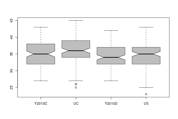
Title produced by software

Notched Boxplots

Date of computation

Sat, 09 Oct 2010 11:52:59 +0000

Cite this page as follows

Statistical Computations at FreeStatistics.org, Office for Research Development and Education, URL https://freestatistics.org/blog/index.php?v=date/2010/Oct/09/t1286625139j28i9sfudjhbeej.htm/, Retrieved Mon, 29 Apr 2024 01:23:55 +0000

Statistical Computations at FreeStatistics.org, Office for Research Development and Education, URL https://freestatistics.org/blog/index.php?pk=82116, Retrieved Mon, 29 Apr 2024 01:23:55 +0000

QR Codes:

Paste this QR Code to cite your computation.

Original text written by user:

IsPrivate?

No (this computation is public)

User-defined keywords

Estimated Impact

220

Family? (F = Feedback message, R = changed R code, M = changed R Module, P = changed Parameters, D = changed Data)

-     [Survey Scores] [E-Learn 2008 table 1] [2008-09-07 11:33:54] [b98453cac15ba1066b407e146608df68]
F RM D  [Survey Scores] [ATTLES] [2010-04-05 12:47:13] [b98453cac15ba1066b407e146608df68]
F RMPD    [Notched Boxplots] [Compare ATTLES Sc...] [2010-10-03 17:09:07] [b98453cac15ba1066b407e146608df68]
F             [Notched Boxplots] [] [2010-10-09 11:52:59] [a7dcbcc9dd9573c89c41df6a7f8b5a0d] [Current]
- R             [Notched Boxplots] [workshop 2 Task 6] [2013-10-15 10:22:39] [f661ab64c60045a179a329b9ddab9bfe] 

Feedback Forum

2010-10-17 10:02:45 [201022de16daa1dc0c172603d7d3cd57] [reply] 
Hier is geen verschil te merken. De mediaan verschilt wel 1 punt maar dit is hier niet van belang. Bij een notched boxplot moet je kijken naar de inkepingen, deze stellen de standaarddeviatie voor. Als deze inkepingen elkaar overlappen dan is er geen verschil.
2010-10-17 14:00:39 [6f5a430a34dfbeab884e51a2f2a26434] [reply] 
Je maakt hier een foute conclusie. 
 
Je ziet dat de inkervingen van de notched boxplots elkaar overlappen, wat wil zeggen dat de verschillen tussen de mediaan te wijten zijn aan het toeval. Moesten dan inkervingen elkaar niet overlappen, dan weet men dat het buiten het toeval valt. 
 
Conclusie: er is sprake van connectedness. 

Post a new message

Dataseries X:

Download CSV

Histogram

Boxplots

41	34	38	30
39	33	32	28
30	29	35	31
31	34	33	35
34	32	37	35
35	35	29	37
39	41	31	39
34	27	36	31
36	40	35	38
37	40	38	37
38	36	31	37
36	40	34	35
38	43	35	37
39	40	38	42
33	33	37	28
32	37	33	37
36	32	32	36
38	26	38	37
39	36	38	33
32	39	32	40
32	38	33	30
31	34	31	36
39	35	38	33
37	41	39	40
39	42	32	37
41	36	32	37
36	39	35	39
33	33	37	35
33	33	33	36
34	36	33	34
31	37	28	36
27	36	32	32
37	34	31	33
34	32	37	27
34	35	30	37
32	39	33	32
29	30	31	31
36	25	33	31
29	29	31	32
35	39	33	37
37	31	32	25
34	26	33	30
38	28	32	37
35	40	33	37
38	32	28	40
37	35	35	35
38	32	39	35
33	41	34	43
36	34	38	32
38	36	32	42
32	38	38	35
32	34	30	27
32	32	33	30
34	34	38	31
32	32	32	36
37	40	32	36
39	43	34	41
29	35	34	34
37	45	36	36
35	36	34	33
30	39	28	35
38	31	34	28
34	36	35	33
31	36	35	38
34	37	31	37
35	40	37	39
36	35	35	34
30	36	27	32
39	32	40	36
35	36	37	36
38	37	36	35
31	42	38	33
34	37	39	42
38	36	41	36
34	36	27	33
39	33	30	36
37	37	37	32
34	35	31	35
28	37	31	38
37	28	27	33
33	33	36	32
37	45	38	38
35	38	37	39
37	43	33	39
32	37	34	39
33	36	31	30
38	40	39	38
33	39	34	38
29	43	32	42
33	32	33	41
31	37	36	31
36	34	32	39
35	44	41	40
32	35	28	31
29	34	30	34
39	37	36	23
37	40	35	28
35	36	31	36
37	44	34	41
32	35	36	29
38	34	36	31
37	40	35	33
36	34	37	35
32	39	28	35
33	36	39	34
40	40	32	40
38	37	35	34
41	35	39	36
36	45	35	35
43	39	42	39

Summary of computational transaction
Raw Input	view raw input (R code)
Raw Output	view raw output of R engine
Computing time	2 seconds
R Server	'Sir Ronald Aylmer Fisher' @ 193.190.124.24

\begin{tabular}{lllllllll}
\hline
Summary of computational transaction \tabularnewline
Raw Input & view raw input (R code)  \tabularnewline
Raw Output & view raw output of R engine  \tabularnewline
Computing time & 2 seconds \tabularnewline
R Server & 'Sir Ronald Aylmer Fisher' @ 193.190.124.24 \tabularnewline
\hline
\end{tabular}
%Source: https://freestatistics.org/blog/index.php?pk=82116&T=0

[TABLE]
[ROW][C]Summary of computational transaction[/C][/ROW]
[ROW][C]Raw Input[/C][C]view raw input (R code) [/C][/ROW]
[ROW][C]Raw Output[/C][C]view raw output of R engine [/C][/ROW]
[ROW][C]Computing time[/C][C]2 seconds[/C][/ROW]
[ROW][C]R Server[/C][C]'Sir Ronald Aylmer Fisher' @ 193.190.124.24[/C][/ROW]
[/TABLE]
Source: https://freestatistics.org/blog/index.php?pk=82116&T=0

Globally Unique Identifier (entire table): ba.freestatistics.org/blog/index.php?pk=82116&T=0

As an alternative you can also use a QR Code:

The GUIDs for individual cells are displayed in the table below:

Summary of computational transaction
Raw Input	view raw input (R code)
Raw Output	view raw output of R engine
Computing time	2 seconds
R Server	'Sir Ronald Aylmer Fisher' @ 193.190.124.24

Boxplot statistics
Variable	lower whisker	lower hinge	median	upper hinge	upper whisker
Y2010C	27	32	35	38	43
UC	27	34	36	39	45
Y2010S	27	32	34	37	42
US	25	32	35	37	43

\begin{tabular}{lllllllll}
\hline
Boxplot statistics \tabularnewline
Variable & lower whisker & lower hinge & median & upper hinge & upper whisker \tabularnewline
Y2010C & 27 & 32 & 35 & 38 & 43 \tabularnewline
UC & 27 & 34 & 36 & 39 & 45 \tabularnewline
Y2010S & 27 & 32 & 34 & 37 & 42 \tabularnewline
US & 25 & 32 & 35 & 37 & 43 \tabularnewline
\hline
\end{tabular}
%Source: https://freestatistics.org/blog/index.php?pk=82116&T=1

[TABLE]
[ROW][C]Boxplot statistics[/C][/ROW]
[ROW][C]Variable[/C][C]lower whisker[/C][C]lower hinge[/C][C]median[/C][C]upper hinge[/C][C]upper whisker[/C][/ROW]
[ROW][C]Y2010C[/C][C]27[/C][C]32[/C][C]35[/C][C]38[/C][C]43[/C][/ROW]
[ROW][C]UC[/C][C]27[/C][C]34[/C][C]36[/C][C]39[/C][C]45[/C][/ROW]
[ROW][C]Y2010S[/C][C]27[/C][C]32[/C][C]34[/C][C]37[/C][C]42[/C][/ROW]
[ROW][C]US[/C][C]25[/C][C]32[/C][C]35[/C][C]37[/C][C]43[/C][/ROW]
[/TABLE]
Source: https://freestatistics.org/blog/index.php?pk=82116&T=1

Globally Unique Identifier (entire table): ba.freestatistics.org/blog/index.php?pk=82116&T=1

As an alternative you can also use a QR Code:

The GUIDs for individual cells are displayed in the table below:

Boxplot statistics
Variable	lower whisker	lower hinge	median	upper hinge	upper whisker
Y2010C	27	32	35	38	43
UC	27	34	36	39	45
Y2010S	27	32	34	37	42
US	25	32	35	37	43

Boxplot Notches
Variable	lower bound	median	upper bound
Y2010C	34.0961174653952	35	35.9038825346048
UC	35.246764554496	36	36.753235445504
Y2010S	33.246764554496	34	34.753235445504
US	34.246764554496	35	35.753235445504

\begin{tabular}{lllllllll}
\hline
Boxplot Notches \tabularnewline
Variable & lower bound & median & upper bound \tabularnewline
Y2010C & 34.0961174653952 & 35 & 35.9038825346048 \tabularnewline
UC & 35.246764554496 & 36 & 36.753235445504 \tabularnewline
Y2010S & 33.246764554496 & 34 & 34.753235445504 \tabularnewline
US & 34.246764554496 & 35 & 35.753235445504 \tabularnewline
\hline
\end{tabular}
%Source: https://freestatistics.org/blog/index.php?pk=82116&T=2

[TABLE]
[ROW][C]Boxplot Notches[/C][/ROW]
[ROW][C]Variable[/C][C]lower bound[/C][C]median[/C][C]upper bound[/C][/ROW]
[ROW][C]Y2010C[/C][C]34.0961174653952[/C][C]35[/C][C]35.9038825346048[/C][/ROW]
[ROW][C]UC[/C][C]35.246764554496[/C][C]36[/C][C]36.753235445504[/C][/ROW]
[ROW][C]Y2010S[/C][C]33.246764554496[/C][C]34[/C][C]34.753235445504[/C][/ROW]
[ROW][C]US[/C][C]34.246764554496[/C][C]35[/C][C]35.753235445504[/C][/ROW]
[/TABLE]
Source: https://freestatistics.org/blog/index.php?pk=82116&T=2

Globally Unique Identifier (entire table): ba.freestatistics.org/blog/index.php?pk=82116&T=2

As an alternative you can also use a QR Code:

The GUIDs for individual cells are displayed in the table below:

Boxplot Notches
Variable	lower bound	median	upper bound
Y2010C	34.0961174653952	35	35.9038825346048
UC	35.246764554496	36	36.753235445504
Y2010S	33.246764554496	34	34.753235445504
US	34.246764554496	35	35.753235445504

Figure 1

PNG link

Postscript link

PDF link

Parameters (Session):

par1 = grey ;

Parameters (R input):

par1 = grey ; par2 = ; par3 = ; par4 = ; par5 = ; par6 = ; par7 = ; par8 = ; par9 = ; par10 = ; par11 = ; par12 = ; par13 = ; par14 = ; par15 = ; par16 = ; par17 = ; par18 = ; par19 = ; par20 = ;

R code (references can be found in the software module):

z <- as.data.frame(t(y))
bitmap(file='test1.png')
(r<-boxplot(z ,xlab=xlab,ylab=ylab,main=main,notch=TRUE,col=par1))
dev.off()
load(file='createtable')
a<-table.start()
a<-table.row.start(a)
a<-table.element(a,hyperlink('overview.htm','Boxplot statistics','Boxplot overview'),6,TRUE)
a<-table.row.end(a)
a<-table.row.start(a)
a<-table.element(a,'Variable',1,TRUE)
a<-table.element(a,hyperlink('lower_whisker.htm','lower whisker','definition of lower whisker'),1,TRUE)
a<-table.element(a,hyperlink('lower_hinge.htm','lower hinge','definition of lower hinge'),1,TRUE)
a<-table.element(a,hyperlink('central_tendency.htm','median','definitions about measures of central tendency'),1,TRUE)
a<-table.element(a,hyperlink('upper_hinge.htm','upper hinge','definition of upper hinge'),1,TRUE)
a<-table.element(a,hyperlink('upper_whisker.htm','upper whisker','definition of upper whisker'),1,TRUE)
a<-table.row.end(a)
for (i in 1:length(y[,1]))
{
a<-table.row.start(a)
a<-table.element(a,dimnames(t(x))[[2]][i],1,TRUE)
for (j in 1:5)
{
a<-table.element(a,r$stats[j,i])
}
a<-table.row.end(a)
}
a<-table.end(a)
table.save(a,file='mytable.tab')
a<-table.start()
a<-table.row.start(a)
a<-table.element(a,'Boxplot Notches',4,TRUE)
a<-table.row.end(a)
a<-table.row.start(a)
a<-table.element(a,'Variable',1,TRUE)
a<-table.element(a,'lower bound',1,TRUE)
a<-table.element(a,'median',1,TRUE)
a<-table.element(a,'upper bound',1,TRUE)
a<-table.row.end(a)
for (i in 1:length(y[,1]))
{
a<-table.row.start(a)
a<-table.element(a,dimnames(t(x))[[2]][i],1,TRUE)
a<-table.element(a,r$conf[1,i])
a<-table.element(a,r$stats[3,i])
a<-table.element(a,r$conf[2,i])
a<-table.row.end(a)
}
a<-table.end(a)
table.save(a,file='mytable1.tab')

Free Statistics

Description of Statistical Computation

Tree of Dependent Computations

Dataset

Tables (Output of Computation)

Figures (Output of Computation)

Input Parameters & R Code