Free Statistics
of Irreproducible Research!
Description of Statistical Computation | |||||||||||||||||||||||||||||||||||||||||||||||||||||||||||||
|---|---|---|---|---|---|---|---|---|---|---|---|---|---|---|---|---|---|---|---|---|---|---|---|---|---|---|---|---|---|---|---|---|---|---|---|---|---|---|---|---|---|---|---|---|---|---|---|---|---|---|---|---|---|---|---|---|---|---|---|---|---|
| Author's title | |||||||||||||||||||||||||||||||||||||||||||||||||||||||||||||
| Author | *The author of this computation has been verified* | ||||||||||||||||||||||||||||||||||||||||||||||||||||||||||||
| R Software Module | rwasp_linear_regression.wasp | ||||||||||||||||||||||||||||||||||||||||||||||||||||||||||||
| Title produced by software | Linear Regression Graphical Model Validation | ||||||||||||||||||||||||||||||||||||||||||||||||||||||||||||
| Date of computation | Tue, 30 Nov 2010 22:15:19 +0000 | ||||||||||||||||||||||||||||||||||||||||||||||||||||||||||||
| Cite this page as follows | Statistical Computations at FreeStatistics.org, Office for Research Development and Education, URL https://freestatistics.org/blog/index.php?v=date/2010/Nov/30/t129115527546dprz9w198l287.htm/, Retrieved Mon, 29 Apr 2024 09:18:57 +0000 | ||||||||||||||||||||||||||||||||||||||||||||||||||||||||||||
| Statistical Computations at FreeStatistics.org, Office for Research Development and Education, URL https://freestatistics.org/blog/index.php?pk=103842, Retrieved Mon, 29 Apr 2024 09:18:57 +0000 | |||||||||||||||||||||||||||||||||||||||||||||||||||||||||||||
| QR Codes: | |||||||||||||||||||||||||||||||||||||||||||||||||||||||||||||
|
| |||||||||||||||||||||||||||||||||||||||||||||||||||||||||||||
| Original text written by user: | |||||||||||||||||||||||||||||||||||||||||||||||||||||||||||||
| IsPrivate? | No (this computation is public) | ||||||||||||||||||||||||||||||||||||||||||||||||||||||||||||
| User-defined keywords | |||||||||||||||||||||||||||||||||||||||||||||||||||||||||||||
| Estimated Impact | 128 | ||||||||||||||||||||||||||||||||||||||||||||||||||||||||||||
Tree of Dependent Computations | |||||||||||||||||||||||||||||||||||||||||||||||||||||||||||||
| Family? (F = Feedback message, R = changed R code, M = changed R Module, P = changed Parameters, D = changed Data) | |||||||||||||||||||||||||||||||||||||||||||||||||||||||||||||
| - [Linear Regression Graphical Model Validation] [Colombia Coffee -...] [2008-02-26 10:22:06] [74be16979710d4c4e7c6647856088456] - M D [Linear Regression Graphical Model Validation] [] [2010-11-25 09:23:05] [4dfa50539945b119a90a7606969443b9] - D [Linear Regression Graphical Model Validation] [Paper - Autocorre...] [2010-11-30 21:57:38] [8677c3f87cec9201607d40be65aa9670] - D [Linear Regression Graphical Model Validation] [Paper - Autocorre...] [2010-11-30 22:15:19] [ffc0b3af89e3f152a248771909785efd] [Current] | |||||||||||||||||||||||||||||||||||||||||||||||||||||||||||||
| Feedback Forum | |||||||||||||||||||||||||||||||||||||||||||||||||||||||||||||
Post a new message | |||||||||||||||||||||||||||||||||||||||||||||||||||||||||||||
Dataset | |||||||||||||||||||||||||||||||||||||||||||||||||||||||||||||
| Dataseries X: | |||||||||||||||||||||||||||||||||||||||||||||||||||||||||||||
162556 29790 87550 84738 54660 42634 40949 45187 37704 16275 25830 12679 18014 43556 24811 6575 7123 21950 37597 17821 12988 22330 13326 16189 7146 15824 27664 11920 8568 14416 3369 11819 6984 4519 2220 18562 10327 5336 2365 4069 8636 13718 4525 6869 4628 3689 4891 7489 4901 2284 3160 4150 7285 1134 4658 2384 3748 5371 1285 9327 5565 1528 3122 7561 2675 13253 880 2053 1424 4036 3045 5119 1431 554 1975 1765 1012 810 1280 666 1380 4677 876 814 514 5692 3642 540 2099 567 2001 2949 2253 6533 1889 3055 272 1414 2564 1383 | |||||||||||||||||||||||||||||||||||||||||||||||||||||||||||||
| Dataseries Y: | |||||||||||||||||||||||||||||||||||||||||||||||||||||||||||||
6282154 4321023 4111912 223193 1491348 1629616 1398893 1926517 983660 1443586 1073089 984885 1405225 227132 929118 1071292 638830 856956 992426 444477 857217 711969 702380 358589 297978 585715 657954 209458 786690 439798 688779 574339 741409 597793 644190 377934 640273 697458 550608 207393 301607 345783 501749 379983 387475 377305 370837 430866 469107 194493 530670 518365 491303 527021 233773 405972 652925 446211 341340 387699 493408 146494 414462 364304 355178 357760 261216 397144 374943 424898 202055 378525 310768 325738 394510 247060 368078 236761 312378 339836 347385 426280 352850 301881 377516 357312 458343 354228 308636 386212 393343 378509 452469 364839 358649 376641 429112 330546 403560 317892 | |||||||||||||||||||||||||||||||||||||||||||||||||||||||||||||
Tables (Output of Computation) | |||||||||||||||||||||||||||||||||||||||||||||||||||||||||||||
| |||||||||||||||||||||||||||||||||||||||||||||||||||||||||||||
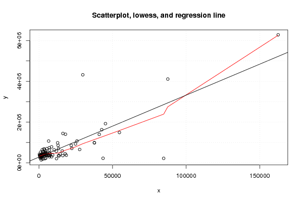
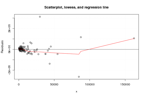
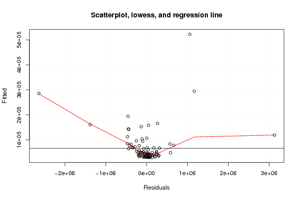
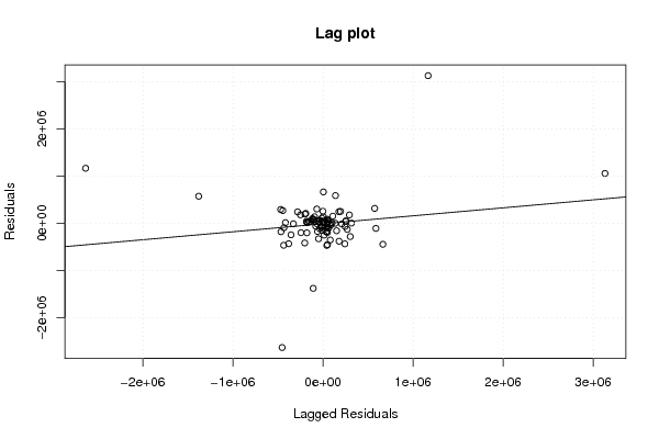
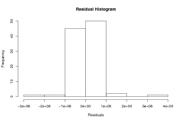
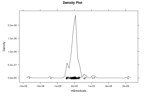
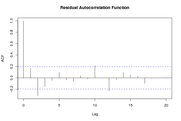
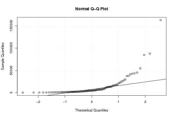
Figures (Output of Computation) | |||||||||||||||||||||||||||||||||||||||||||||||||||||||||||||
Input Parameters & R Code | |||||||||||||||||||||||||||||||||||||||||||||||||||||||||||||
| Parameters (Session): | |||||||||||||||||||||||||||||||||||||||||||||||||||||||||||||
| par1 = 0 ; | |||||||||||||||||||||||||||||||||||||||||||||||||||||||||||||
| Parameters (R input): | |||||||||||||||||||||||||||||||||||||||||||||||||||||||||||||
| par1 = 0 ; | |||||||||||||||||||||||||||||||||||||||||||||||||||||||||||||
| R code (references can be found in the software module): | |||||||||||||||||||||||||||||||||||||||||||||||||||||||||||||
par1 <- as.numeric(par1) | |||||||||||||||||||||||||||||||||||||||||||||||||||||||||||||