Free Statistics
of Irreproducible Research!
Description of Statistical Computation | |||||||||||||||||||||
|---|---|---|---|---|---|---|---|---|---|---|---|---|---|---|---|---|---|---|---|---|---|
| Author's title | |||||||||||||||||||||
| Author | *The author of this computation has been verified* | ||||||||||||||||||||
| R Software Module | rwasp_meanplot.wasp | ||||||||||||||||||||
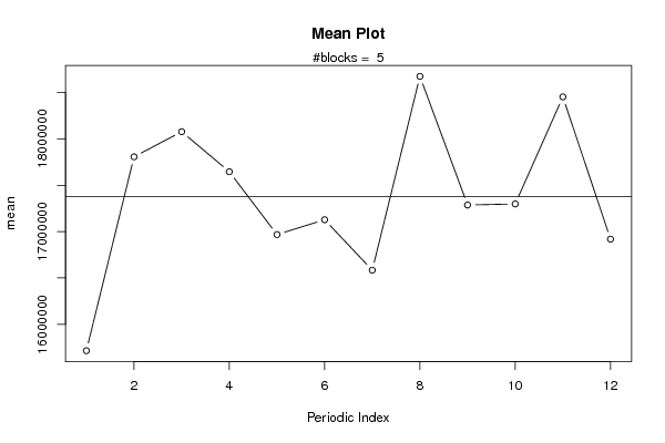
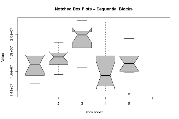
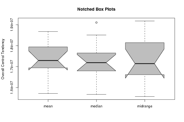
| Title produced by software | Mean Plot | ||||||||||||||||||||
| Date of computation | Tue, 30 Nov 2010 15:31:42 +0000 | ||||||||||||||||||||
| Cite this page as follows | Statistical Computations at FreeStatistics.org, Office for Research Development and Education, URL https://freestatistics.org/blog/index.php?v=date/2010/Nov/30/t12911309851so73v5paf3zd1h.htm/, Retrieved Mon, 29 Apr 2024 13:24:03 +0000 | ||||||||||||||||||||
| Statistical Computations at FreeStatistics.org, Office for Research Development and Education, URL https://freestatistics.org/blog/index.php?pk=103618, Retrieved Mon, 29 Apr 2024 13:24:03 +0000 | |||||||||||||||||||||
| QR Codes: | |||||||||||||||||||||
|
| |||||||||||||||||||||
| Original text written by user: | |||||||||||||||||||||
| IsPrivate? | No (this computation is public) | ||||||||||||||||||||
| User-defined keywords | |||||||||||||||||||||
| Estimated Impact | 111 | ||||||||||||||||||||
Tree of Dependent Computations | |||||||||||||||||||||
| Family? (F = Feedback message, R = changed R code, M = changed R Module, P = changed Parameters, D = changed Data) | |||||||||||||||||||||
| - [Bivariate Data Series] [Bivariate dataset] [2008-01-05 23:51:08] [74be16979710d4c4e7c6647856088456] F RMPD [Mean Plot] [Colombia Coffee] [2008-01-07 13:38:24] [74be16979710d4c4e7c6647856088456] - MPD [Mean Plot] [Paper Mean plot e...] [2010-11-30 15:31:42] [9d72585f2b7b60ae977d4816136e1c95] [Current] | |||||||||||||||||||||
| Feedback Forum | |||||||||||||||||||||
Post a new message | |||||||||||||||||||||
Dataset | |||||||||||||||||||||
| Dataseries X: | |||||||||||||||||||||
14731798,37 16471559,62 15213975,95 17637387,4 17972385,83 16896235,55 16697955,94 19691579,52 15930700,75 17444615,98 17699369,88 15189796,81 15672722,75 17180794,3 17664893,45 17862884,98 16162288,88 17463628,82 16772112,17 19106861,48 16721314,25 18161267,85 18509941,2 17802737,97 16409869,75 17967742,04 20286602,27 19537280,81 18021889,62 20194317,23 19049596,62 20244720,94 21473302,24 19673603,19 21053177,29 20159479,84 18203628,31 21289464,94 20432335,71 17180395,07 15816786,32 15071819,75 14521120,61 15668789,39 14346884,11 13881008,13 15465943,69 14238232,92 13557713,21 16127590,29 16793894,2 16014007,43 16867867,15 16014583,21 15878594,85 18664899,14 17962530,06 17332692,2 19542066,35 17203555,19 | |||||||||||||||||||||
Tables (Output of Computation) | |||||||||||||||||||||
| |||||||||||||||||||||
Figures (Output of Computation) | |||||||||||||||||||||
Input Parameters & R Code | |||||||||||||||||||||
| Parameters (Session): | |||||||||||||||||||||
| par1 = 12 ; | |||||||||||||||||||||
| Parameters (R input): | |||||||||||||||||||||
| par1 = 12 ; | |||||||||||||||||||||
| R code (references can be found in the software module): | |||||||||||||||||||||
par1 <- as.numeric(par1) | |||||||||||||||||||||