Free Statistics
of Irreproducible Research!
Description of Statistical Computation | |||||||||||||||||||||||||||||||||||||||||||||||||||||||||||||
|---|---|---|---|---|---|---|---|---|---|---|---|---|---|---|---|---|---|---|---|---|---|---|---|---|---|---|---|---|---|---|---|---|---|---|---|---|---|---|---|---|---|---|---|---|---|---|---|---|---|---|---|---|---|---|---|---|---|---|---|---|---|
| Author's title | |||||||||||||||||||||||||||||||||||||||||||||||||||||||||||||
| Author | *The author of this computation has been verified* | ||||||||||||||||||||||||||||||||||||||||||||||||||||||||||||
| R Software Module | rwasp_linear_regression.wasp | ||||||||||||||||||||||||||||||||||||||||||||||||||||||||||||
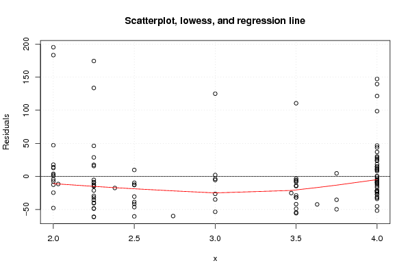
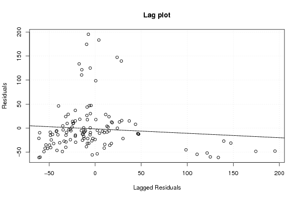
| Title produced by software | Linear Regression Graphical Model Validation | ||||||||||||||||||||||||||||||||||||||||||||||||||||||||||||
| Date of computation | Fri, 26 Nov 2010 19:43:47 +0000 | ||||||||||||||||||||||||||||||||||||||||||||||||||||||||||||
| Cite this page as follows | Statistical Computations at FreeStatistics.org, Office for Research Development and Education, URL https://freestatistics.org/blog/index.php?v=date/2010/Nov/26/t1290800603halqlcsfqcoladf.htm/, Retrieved Fri, 03 May 2024 15:47:02 +0000 | ||||||||||||||||||||||||||||||||||||||||||||||||||||||||||||
| Statistical Computations at FreeStatistics.org, Office for Research Development and Education, URL https://freestatistics.org/blog/index.php?pk=102167, Retrieved Fri, 03 May 2024 15:47:02 +0000 | |||||||||||||||||||||||||||||||||||||||||||||||||||||||||||||
| QR Codes: | |||||||||||||||||||||||||||||||||||||||||||||||||||||||||||||
|
| |||||||||||||||||||||||||||||||||||||||||||||||||||||||||||||
| Original text written by user: | |||||||||||||||||||||||||||||||||||||||||||||||||||||||||||||
| IsPrivate? | No (this computation is public) | ||||||||||||||||||||||||||||||||||||||||||||||||||||||||||||
| User-defined keywords | |||||||||||||||||||||||||||||||||||||||||||||||||||||||||||||
| Estimated Impact | 126 | ||||||||||||||||||||||||||||||||||||||||||||||||||||||||||||
Tree of Dependent Computations | |||||||||||||||||||||||||||||||||||||||||||||||||||||||||||||
| Family? (F = Feedback message, R = changed R code, M = changed R Module, P = changed Parameters, D = changed Data) | |||||||||||||||||||||||||||||||||||||||||||||||||||||||||||||
| - [Linear Regression Graphical Model Validation] [Colombia Coffee -...] [2008-02-26 10:22:06] [74be16979710d4c4e7c6647856088456] - M D [Linear Regression Graphical Model Validation] [] [2010-11-26 19:43:47] [3213ed9efdb724e3c847d204cd8135dd] [Current] | |||||||||||||||||||||||||||||||||||||||||||||||||||||||||||||
| Feedback Forum | |||||||||||||||||||||||||||||||||||||||||||||||||||||||||||||
Post a new message | |||||||||||||||||||||||||||||||||||||||||||||||||||||||||||||
Dataset | |||||||||||||||||||||||||||||||||||||||||||||||||||||||||||||
| Dataseries X: | |||||||||||||||||||||||||||||||||||||||||||||||||||||||||||||
2.00 2.00 2.00 2.00 2.00 2.00 2.00 2.00 2.00 2.00 2.00 2.00 2.00 2.00 2.03 2.25 2.25 2.25 2.25 2.25 2.25 2.25 2.25 2.25 2.25 2.25 2.25 2.25 2.25 2.25 2.25 2.25 2.25 2.25 2.25 2.25 2.25 2.38 2.50 2.50 2.50 2.50 2.50 2.50 2.50 2.50 2.50 2.74 3.00 3.00 3.00 3.00 3.00 3.00 3.00 3.47 3.50 3.50 3.50 3.50 3.50 3.50 3.50 3.50 3.50 3.50 3.50 3.50 3.50 3.50 3.63 4.00 4.00 4.00 4.00 4.00 4.00 4.00 4.00 4.00 4.00 4.00 4.00 4.00 4.00 4.00 4.00 4.00 4.00 4.00 4.00 4.00 4.00 4.00 4.00 4.00 4.00 4.00 4.00 4.00 4.00 4.00 4.00 4.00 4.00 4.00 4.00 4.00 4.00 4.00 4.00 4.00 4.00 4.00 4.00 4.00 4.00 3.75 3.75 3.75 | |||||||||||||||||||||||||||||||||||||||||||||||||||||||||||||
| Dataseries Y: | |||||||||||||||||||||||||||||||||||||||||||||||||||||||||||||
406,9 227,6 236,4 241,4 224,3 211,1 270,8 219,1 225,9 237,6 199,1 175,9 418,8 216,2 211,6 264,8 178,8 186,7 236,2 210,1 206,2 204,8 178,1 170,3 393,0 209,3 213,4 203,6 170,0 183,0 234,4 247,4 189,3 197,4 157,5 157,6 352,3 198,6 201,2 200,6 167,3 172,1 223,4 183,2 175,1 204,1 153,3 149,0 328,6 198,2 177,3 200,0 168,8 150,2 205,8 169,1 179,8 188,1 151,8 139,2 304,2 178,9 161,9 185,1 144,8 138,0 190,4 165,0 161,9 186,7 148,8 131,9 305,1 169,1 162,1 181,1 156,6 149,8 194,0 160,0 183,5 207,7 151,6 138,5 282,2 184,2 178,2 198,7 162,0 171,5 230,4 177,2 191,6 227,4 174,8 152,5 330,9 207,4 198,6 220,6 162,0 175,5 196,5 210,0 174,6 193,4 159,6 156,7 323,2 212,0 195,0 202,1 166,9 162,0 213,8 178,4 173,0 193,3 153,4 139,0 | |||||||||||||||||||||||||||||||||||||||||||||||||||||||||||||
Tables (Output of Computation) | |||||||||||||||||||||||||||||||||||||||||||||||||||||||||||||
| |||||||||||||||||||||||||||||||||||||||||||||||||||||||||||||
Figures (Output of Computation) | |||||||||||||||||||||||||||||||||||||||||||||||||||||||||||||
Input Parameters & R Code | |||||||||||||||||||||||||||||||||||||||||||||||||||||||||||||
| Parameters (Session): | |||||||||||||||||||||||||||||||||||||||||||||||||||||||||||||
| par1 = 0 ; | |||||||||||||||||||||||||||||||||||||||||||||||||||||||||||||
| Parameters (R input): | |||||||||||||||||||||||||||||||||||||||||||||||||||||||||||||
| par1 = 0 ; | |||||||||||||||||||||||||||||||||||||||||||||||||||||||||||||
| R code (references can be found in the software module): | |||||||||||||||||||||||||||||||||||||||||||||||||||||||||||||
par1 <- as.numeric(par1) | |||||||||||||||||||||||||||||||||||||||||||||||||||||||||||||