Repository of Reproducible Computations

Free Statistics

of Irreproducible Research!

Author's title

Author

*The author of this computation has been verified*

R Software Module

rwasp_meanversusmedian.wasp

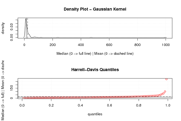
Title produced by software

Mean versus Median

Date of computation

Fri, 26 Nov 2010 14:32:24 +0000

Cite this page as follows

Statistical Computations at FreeStatistics.org, Office for Research Development and Education, URL https://freestatistics.org/blog/index.php?v=date/2010/Nov/26/t12907818982gns973vwk4987i.htm/, Retrieved Sat, 04 May 2024 05:25:56 +0000

Statistical Computations at FreeStatistics.org, Office for Research Development and Education, URL https://freestatistics.org/blog/index.php?pk=101933, Retrieved Sat, 04 May 2024 05:25:56 +0000

QR Codes:

Paste this QR Code to cite your computation.

Original text written by user:

IsPrivate?

No (this computation is public)

User-defined keywords

Estimated Impact

128

Family? (F = Feedback message, R = changed R code, M = changed R Module, P = changed Parameters, D = changed Data)

-       [Mean versus Median] [] [2010-11-26 14:32:24] [c8b0d20ebafa6d61ca10522fa626ae82] [Current]

Feedback Forum

Post a new message

Dataseries X:

Download CSV

Histogram

Boxplots

Summary of computational transaction
Raw Input	view raw input (R code)
Raw Output	view raw output of R engine
Computing time	2 seconds
R Server	'George Udny Yule' @ 72.249.76.132

\begin{tabular}{lllllllll}
\hline
Summary of computational transaction \tabularnewline
Raw Input & view raw input (R code)  \tabularnewline
Raw Output & view raw output of R engine  \tabularnewline
Computing time & 2 seconds \tabularnewline
R Server & 'George Udny Yule' @ 72.249.76.132 \tabularnewline
\hline
\end{tabular}
%Source: https://freestatistics.org/blog/index.php?pk=101933&T=0

[TABLE]
[ROW][C]Summary of computational transaction[/C][/ROW]
[ROW][C]Raw Input[/C][C]view raw input (R code) [/C][/ROW]
[ROW][C]Raw Output[/C][C]view raw output of R engine [/C][/ROW]
[ROW][C]Computing time[/C][C]2 seconds[/C][/ROW]
[ROW][C]R Server[/C][C]'George Udny Yule' @ 72.249.76.132[/C][/ROW]
[/TABLE]
Source: https://freestatistics.org/blog/index.php?pk=101933&T=0

Globally Unique Identifier (entire table): ba.freestatistics.org/blog/index.php?pk=101933&T=0

As an alternative you can also use a QR Code:

The GUIDs for individual cells are displayed in the table below:

Summary of computational transaction
Raw Input	view raw input (R code)
Raw Output	view raw output of R engine
Computing time	2 seconds
R Server	'George Udny Yule' @ 72.249.76.132

Median versus Mean
mean	23.5114253246753
median	13.99

\begin{tabular}{lllllllll}
\hline
Median versus Mean \tabularnewline
mean & 23.5114253246753 \tabularnewline
median & 13.99 \tabularnewline
\hline
\end{tabular}
%Source: https://freestatistics.org/blog/index.php?pk=101933&T=1

[TABLE]
[ROW][C]Median versus Mean[/C][/ROW]
[ROW][C]mean[/C][C]23.5114253246753[/C][/ROW]
[ROW][C]median[/C][C]13.99[/C][/ROW]
[/TABLE]
Source: https://freestatistics.org/blog/index.php?pk=101933&T=1

Globally Unique Identifier (entire table): ba.freestatistics.org/blog/index.php?pk=101933&T=1

As an alternative you can also use a QR Code:

The GUIDs for individual cells are displayed in the table below:

Median versus Mean
mean	23.5114253246753
median	13.99

Figure 1

PNG link

Postscript link

PDF link

Parameters (Session):

Parameters (R input):

R code (references can be found in the software module):

library(Hmisc)
m <- mean(x)
e <- median(x)
bitmap(file='test1.png')
op <- par(mfrow=c(2,1))
mydensity1 <- density(x,kernel='gaussian',na.rm=TRUE)
plot(mydensity1,main='Density Plot - Gaussian Kernel',xlab='Median (0 -> full line) | Mean (0 -> dashed line)',ylab='density')
abline(v=e,lty=1)
abline(v=m,lty=5)
grid()
myseq <- seq(0.01, 0.99, 0.01)
hd <- hdquantile(x, probs = myseq, se = TRUE, na.rm = FALSE, names = TRUE, weights=FALSE)
plot(myseq,hd,col=2,main='Harrell-Davis Quantiles',xlab='quantiles',ylab='Median (0 -> full) | Mean (0 -> dashed)')
abline(h=m,lty=5)
abline(h=e,lty=1)
grid()
par(op)
dev.off()
load(file='createtable')
a<-table.start()
a<-table.row.start(a)
a<-table.element(a,'Median versus Mean',2,TRUE)
a<-table.row.end(a)
a<-table.row.start(a)
a<-table.element(a,'mean',header=TRUE)
a<-table.element(a,mean(x))
a<-table.row.end(a)
a<-table.row.start(a)
a<-table.element(a,'median',header=TRUE)
a<-table.element(a,median(x))
a<-table.row.end(a)
a<-table.end(a)
table.save(a,file='mytable.tab')

Free Statistics

Description of Statistical Computation

Tree of Dependent Computations

Dataset

Tables (Output of Computation)

Figures (Output of Computation)

Input Parameters & R Code