Free Statistics
of Irreproducible Research!
Description of Statistical Computation | |||||||||||||||||||||||||||||||||||||||||||||||||||||||||||||
|---|---|---|---|---|---|---|---|---|---|---|---|---|---|---|---|---|---|---|---|---|---|---|---|---|---|---|---|---|---|---|---|---|---|---|---|---|---|---|---|---|---|---|---|---|---|---|---|---|---|---|---|---|---|---|---|---|---|---|---|---|---|
| Author's title | |||||||||||||||||||||||||||||||||||||||||||||||||||||||||||||
| Author | *The author of this computation has been verified* | ||||||||||||||||||||||||||||||||||||||||||||||||||||||||||||
| R Software Module | rwasp_linear_regression.wasp | ||||||||||||||||||||||||||||||||||||||||||||||||||||||||||||
| Title produced by software | Linear Regression Graphical Model Validation | ||||||||||||||||||||||||||||||||||||||||||||||||||||||||||||
| Date of computation | Fri, 26 Nov 2010 08:07:40 +0000 | ||||||||||||||||||||||||||||||||||||||||||||||||||||||||||||
| Cite this page as follows | Statistical Computations at FreeStatistics.org, Office for Research Development and Education, URL https://freestatistics.org/blog/index.php?v=date/2010/Nov/26/t12907587446xpjkun5v515sa8.htm/, Retrieved Fri, 03 May 2024 17:14:28 +0000 | ||||||||||||||||||||||||||||||||||||||||||||||||||||||||||||
| Statistical Computations at FreeStatistics.org, Office for Research Development and Education, URL https://freestatistics.org/blog/index.php?pk=101694, Retrieved Fri, 03 May 2024 17:14:28 +0000 | |||||||||||||||||||||||||||||||||||||||||||||||||||||||||||||
| QR Codes: | |||||||||||||||||||||||||||||||||||||||||||||||||||||||||||||
|
| |||||||||||||||||||||||||||||||||||||||||||||||||||||||||||||
| Original text written by user: | |||||||||||||||||||||||||||||||||||||||||||||||||||||||||||||
| IsPrivate? | No (this computation is public) | ||||||||||||||||||||||||||||||||||||||||||||||||||||||||||||
| User-defined keywords | |||||||||||||||||||||||||||||||||||||||||||||||||||||||||||||
| Estimated Impact | 108 | ||||||||||||||||||||||||||||||||||||||||||||||||||||||||||||
Tree of Dependent Computations | |||||||||||||||||||||||||||||||||||||||||||||||||||||||||||||
| Family? (F = Feedback message, R = changed R code, M = changed R Module, P = changed Parameters, D = changed Data) | |||||||||||||||||||||||||||||||||||||||||||||||||||||||||||||
| - [Multiple Regression] [Q1 The Seatbeltlaw] [2007-11-14 19:27:43] [8cd6641b921d30ebe00b648d1481bba0] - RMPD [Multiple Regression] [Seatbelt] [2009-11-12 13:54:52] [b98453cac15ba1066b407e146608df68] - RMPD [Linear Regression Graphical Model Validation] [] [2010-11-26 08:07:40] [33c49f0356cf94839cc9a2df1ea19a67] [Current] - D [Linear Regression Graphical Model Validation] [] [2010-11-26 11:56:32] [eab273d59b25a7fddba6574425ce83eb] | |||||||||||||||||||||||||||||||||||||||||||||||||||||||||||||
| Feedback Forum | |||||||||||||||||||||||||||||||||||||||||||||||||||||||||||||
Post a new message | |||||||||||||||||||||||||||||||||||||||||||||||||||||||||||||
Dataset | |||||||||||||||||||||||||||||||||||||||||||||||||||||||||||||
| Dataseries X: | |||||||||||||||||||||||||||||||||||||||||||||||||||||||||||||
825 101 851 1.645 12.952 8.816 3 96 4.942 2.525 311 753 1.433 848 401 145 260 3.213 315 443 914 1.114 268 145 1.909 4.376 3 495 293 1.801 189 799 2.610 10 801 123 662 573 2.086 61 2.199 427 106 254 295 244 79 42 123 1.022 106 192 810 324 75 80 761 1.555 308 55 522 72 399 1.100 31 184 46 376 129 1.260 668 172 | |||||||||||||||||||||||||||||||||||||||||||||||||||||||||||||
| Dataseries Y: | |||||||||||||||||||||||||||||||||||||||||||||||||||||||||||||
1.055 87 892 9.365 11.415 1.219 33 2 13.060 8.642 672 957 1.592 812 882 123 739 1.995 935 636 1.410 619 400 155 1.299 526 2 544 41 2.071 53 3.539 3.605 408 2.177 197 499 1.695 616 26 987 250 195 381 361 383 215 30 446 683 342 251 1.449 255 97 41 552 250 374 14 676 33 2.073 1.491 222 475 87 374 493 324 319 99 | |||||||||||||||||||||||||||||||||||||||||||||||||||||||||||||
Tables (Output of Computation) | |||||||||||||||||||||||||||||||||||||||||||||||||||||||||||||
| |||||||||||||||||||||||||||||||||||||||||||||||||||||||||||||
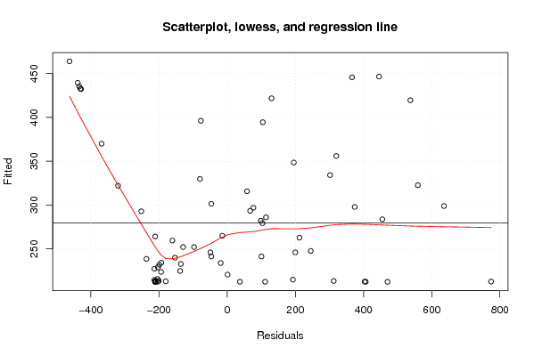
Figures (Output of Computation) | |||||||||||||||||||||||||||||||||||||||||||||||||||||||||||||
Input Parameters & R Code | |||||||||||||||||||||||||||||||||||||||||||||||||||||||||||||
| Parameters (Session): | |||||||||||||||||||||||||||||||||||||||||||||||||||||||||||||
| par1 = 0 ; | |||||||||||||||||||||||||||||||||||||||||||||||||||||||||||||
| Parameters (R input): | |||||||||||||||||||||||||||||||||||||||||||||||||||||||||||||
| par1 = 0 ; | |||||||||||||||||||||||||||||||||||||||||||||||||||||||||||||
| R code (references can be found in the software module): | |||||||||||||||||||||||||||||||||||||||||||||||||||||||||||||
par1 <- as.numeric(par1) | |||||||||||||||||||||||||||||||||||||||||||||||||||||||||||||