Free Statistics
of Irreproducible Research!
Description of Statistical Computation | |||||||||||||||||||||||||||||||||||||||||||||||||||||||||||||
|---|---|---|---|---|---|---|---|---|---|---|---|---|---|---|---|---|---|---|---|---|---|---|---|---|---|---|---|---|---|---|---|---|---|---|---|---|---|---|---|---|---|---|---|---|---|---|---|---|---|---|---|---|---|---|---|---|---|---|---|---|---|
| Author's title | |||||||||||||||||||||||||||||||||||||||||||||||||||||||||||||
| Author | *The author of this computation has been verified* | ||||||||||||||||||||||||||||||||||||||||||||||||||||||||||||
| R Software Module | rwasp_linear_regression.wasp | ||||||||||||||||||||||||||||||||||||||||||||||||||||||||||||
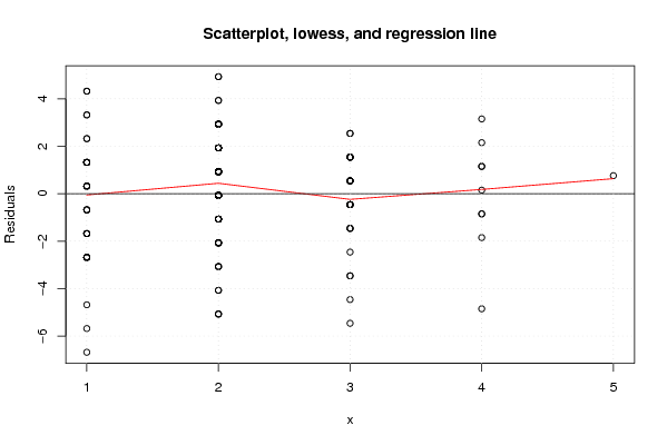
| Title produced by software | Linear Regression Graphical Model Validation | ||||||||||||||||||||||||||||||||||||||||||||||||||||||||||||
| Date of computation | Tue, 16 Nov 2010 18:56:14 +0000 | ||||||||||||||||||||||||||||||||||||||||||||||||||||||||||||
| Cite this page as follows | Statistical Computations at FreeStatistics.org, Office for Research Development and Education, URL https://freestatistics.org/blog/index.php?v=date/2010/Nov/16/t1289933719m8e6ri67k4qma2e.htm/, Retrieved Sun, 05 May 2024 06:52:29 +0000 | ||||||||||||||||||||||||||||||||||||||||||||||||||||||||||||
| Statistical Computations at FreeStatistics.org, Office for Research Development and Education, URL https://freestatistics.org/blog/index.php?pk=96277, Retrieved Sun, 05 May 2024 06:52:29 +0000 | |||||||||||||||||||||||||||||||||||||||||||||||||||||||||||||
| QR Codes: | |||||||||||||||||||||||||||||||||||||||||||||||||||||||||||||
|
| |||||||||||||||||||||||||||||||||||||||||||||||||||||||||||||
| Original text written by user: | |||||||||||||||||||||||||||||||||||||||||||||||||||||||||||||
| IsPrivate? | No (this computation is public) | ||||||||||||||||||||||||||||||||||||||||||||||||||||||||||||
| User-defined keywords | |||||||||||||||||||||||||||||||||||||||||||||||||||||||||||||
| Estimated Impact | 114 | ||||||||||||||||||||||||||||||||||||||||||||||||||||||||||||
Tree of Dependent Computations | |||||||||||||||||||||||||||||||||||||||||||||||||||||||||||||
| Family? (F = Feedback message, R = changed R code, M = changed R Module, P = changed Parameters, D = changed Data) | |||||||||||||||||||||||||||||||||||||||||||||||||||||||||||||
| - [Linear Regression Graphical Model Validation] [Colombia Coffee -...] [2008-02-26 10:22:06] [74be16979710d4c4e7c6647856088456] - M D [Linear Regression Graphical Model Validation] [WS - Minitut] [2010-11-16 00:58:47] [19f9551d4d95750ef21e9f3cf8fe2131] - D [Linear Regression Graphical Model Validation] [mini tut] [2010-11-16 18:38:52] [87116ee6ef949037dfa02b8eb1a3bf97] F D [Linear Regression Graphical Model Validation] [tut] [2010-11-16 18:56:14] [66b4703b90a9701067ac75b10c82aca9] [Current] - D [Linear Regression Graphical Model Validation] [tut 2] [2010-11-16 19:09:07] [87116ee6ef949037dfa02b8eb1a3bf97] | |||||||||||||||||||||||||||||||||||||||||||||||||||||||||||||
| Feedback Forum | |||||||||||||||||||||||||||||||||||||||||||||||||||||||||||||
Post a new message | |||||||||||||||||||||||||||||||||||||||||||||||||||||||||||||
Dataset | |||||||||||||||||||||||||||||||||||||||||||||||||||||||||||||
| Dataseries X: | |||||||||||||||||||||||||||||||||||||||||||||||||||||||||||||
1 4 1 2 3 2 2 1 2 1 2 2 2 2 1 2 4 2 2 2 1 1 2 2 2 2 1 3 2 2 4 3 1 1 2 2 1 1 3 2 2 3 1 1 1 3 3 2 2 1 2 2 1 2 1 3 2 2 1 2 1 2 1 1 2 4 1 2 3 2 4 3 1 1 4 2 2 1 2 2 2 3 4 2 2 2 3 1 2 1 4 3 2 2 3 2 2 3 2 1 2 1 2 1 2 2 5 1 3 2 3 2 2 1 2 3 3 3 3 2 3 3 2 2 1 2 1 3 2 2 1 2 1 1 2 2 2 2 1 1 1 1 4 2 1 2 2 3 1 3 2 2 | |||||||||||||||||||||||||||||||||||||||||||||||||||||||||||||
| Dataseries Y: | |||||||||||||||||||||||||||||||||||||||||||||||||||||||||||||
14 18 11 12 16 18 14 14 15 15 17 19 10 16 18 14 14 17 14 16 18 11 14 12 17 9 16 14 15 11 16 13 17 15 14 16 9 15 17 13 15 16 16 12 12 11 15 15 17 13 16 14 11 12 12 15 16 15 12 12 8 13 11 14 15 10 11 12 15 15 14 16 15 15 13 12 17 13 15 13 15 16 15 16 15 14 15 14 13 7 17 13 15 14 13 16 12 14 17 15 17 12 16 11 15 9 16 15 10 10 15 11 13 14 18 16 14 14 14 14 12 14 15 15 15 13 17 17 19 15 13 9 15 15 15 16 11 14 11 15 13 15 16 14 15 16 16 11 12 9 16 13 | |||||||||||||||||||||||||||||||||||||||||||||||||||||||||||||
Tables (Output of Computation) | |||||||||||||||||||||||||||||||||||||||||||||||||||||||||||||
| |||||||||||||||||||||||||||||||||||||||||||||||||||||||||||||
Figures (Output of Computation) | |||||||||||||||||||||||||||||||||||||||||||||||||||||||||||||
Input Parameters & R Code | |||||||||||||||||||||||||||||||||||||||||||||||||||||||||||||
| Parameters (Session): | |||||||||||||||||||||||||||||||||||||||||||||||||||||||||||||
| par1 = 0 ; | |||||||||||||||||||||||||||||||||||||||||||||||||||||||||||||
| Parameters (R input): | |||||||||||||||||||||||||||||||||||||||||||||||||||||||||||||
| par1 = 0 ; | |||||||||||||||||||||||||||||||||||||||||||||||||||||||||||||
| R code (references can be found in the software module): | |||||||||||||||||||||||||||||||||||||||||||||||||||||||||||||
par1 <- as.numeric(par1) | |||||||||||||||||||||||||||||||||||||||||||||||||||||||||||||