Free Statistics
of Irreproducible Research!
Description of Statistical Computation | |||||||||||||||||||||
|---|---|---|---|---|---|---|---|---|---|---|---|---|---|---|---|---|---|---|---|---|---|
| Author's title | |||||||||||||||||||||
| Author | *The author of this computation has been verified* | ||||||||||||||||||||
| R Software Module | rwasp_meanplot.wasp | ||||||||||||||||||||
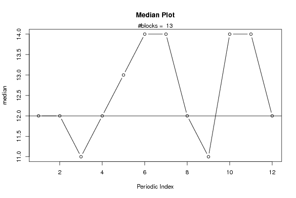
| Title produced by software | Mean Plot | ||||||||||||||||||||
| Date of computation | Tue, 16 Nov 2010 16:34:50 +0000 | ||||||||||||||||||||
| Cite this page as follows | Statistical Computations at FreeStatistics.org, Office for Research Development and Education, URL https://freestatistics.org/blog/index.php?v=date/2010/Nov/16/t1289925207bq94rd7bees4u2k.htm/, Retrieved Sun, 05 May 2024 02:12:02 +0000 | ||||||||||||||||||||
| Statistical Computations at FreeStatistics.org, Office for Research Development and Education, URL https://freestatistics.org/blog/index.php?pk=96038, Retrieved Sun, 05 May 2024 02:12:02 +0000 | |||||||||||||||||||||
| QR Codes: | |||||||||||||||||||||
|
| |||||||||||||||||||||
| Original text written by user: | |||||||||||||||||||||
| IsPrivate? | No (this computation is public) | ||||||||||||||||||||
| User-defined keywords | |||||||||||||||||||||
| Estimated Impact | 116 | ||||||||||||||||||||
Tree of Dependent Computations | |||||||||||||||||||||
| Family? (F = Feedback message, R = changed R code, M = changed R Module, P = changed Parameters, D = changed Data) | |||||||||||||||||||||
| - [Bivariate Data Series] [Bivariate dataset] [2008-01-05 23:51:08] [74be16979710d4c4e7c6647856088456] F RMPD [Mean Plot] [Colombia Coffee] [2008-01-07 13:38:24] [74be16979710d4c4e7c6647856088456] - MPD [Mean Plot] [workshop 6 - tuto...] [2010-11-16 15:22:06] [956e8df26b41c50d9c6c2ec1b6a122a8] - D [Mean Plot] [workshop 6 - tuto...] [2010-11-16 16:34:50] [42b216fecf560ef45cc692f6de9f34dc] [Current] | |||||||||||||||||||||
| Feedback Forum | |||||||||||||||||||||
Post a new message | |||||||||||||||||||||
Dataset | |||||||||||||||||||||
| Dataseries X: | |||||||||||||||||||||
13 12 15 12 10 12 15 9 12 11 11 11 15 7 11 11 10 14 10 6 11 15 11 12 14 15 9 13 13 16 13 12 14 11 9 16 12 10 13 16 14 15 5 8 11 16 17 9 9 13 10 6 12 8 14 12 11 16 8 15 7 16 14 16 9 14 11 13 15 5 15 13 11 11 12 12 12 12 14 6 7 14 14 10 13 12 9 12 16 10 14 10 16 15 12 10 8 8 11 13 16 16 14 11 4 14 9 14 8 8 11 12 11 14 15 16 16 11 14 14 12 14 8 13 16 12 16 12 11 4 16 15 10 13 15 12 14 7 19 12 12 13 15 8 12 10 8 10 15 16 13 16 9 14 14 12 | |||||||||||||||||||||
Tables (Output of Computation) | |||||||||||||||||||||
| |||||||||||||||||||||
Figures (Output of Computation) | |||||||||||||||||||||
Input Parameters & R Code | |||||||||||||||||||||
| Parameters (Session): | |||||||||||||||||||||
| par1 = 12 ; | |||||||||||||||||||||
| Parameters (R input): | |||||||||||||||||||||
| par1 = 12 ; | |||||||||||||||||||||
| R code (references can be found in the software module): | |||||||||||||||||||||
par1 <- as.numeric(par1) | |||||||||||||||||||||