Free Statistics
of Irreproducible Research!
Description of Statistical Computation | |||||||||||||||||||||
|---|---|---|---|---|---|---|---|---|---|---|---|---|---|---|---|---|---|---|---|---|---|
| Author's title | |||||||||||||||||||||
| Author | *Unverified author* | ||||||||||||||||||||
| R Software Module | rwasp_meanplot.wasp | ||||||||||||||||||||
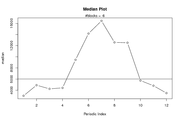
| Title produced by software | Mean Plot | ||||||||||||||||||||
| Date of computation | Tue, 16 Nov 2010 12:59:37 +0000 | ||||||||||||||||||||
| Cite this page as follows | Statistical Computations at FreeStatistics.org, Office for Research Development and Education, URL https://freestatistics.org/blog/index.php?v=date/2010/Nov/16/t12899123734tb85qadfp8c7h4.htm/, Retrieved Sun, 05 May 2024 03:30:01 +0000 | ||||||||||||||||||||
| Statistical Computations at FreeStatistics.org, Office for Research Development and Education, URL https://freestatistics.org/blog/index.php?pk=95603, Retrieved Sun, 05 May 2024 03:30:01 +0000 | |||||||||||||||||||||
| QR Codes: | |||||||||||||||||||||
|
| |||||||||||||||||||||
| Original text written by user: | |||||||||||||||||||||
| IsPrivate? | No (this computation is public) | ||||||||||||||||||||
| User-defined keywords | KDGP1W52 | ||||||||||||||||||||
| Estimated Impact | 103 | ||||||||||||||||||||
Tree of Dependent Computations | |||||||||||||||||||||
| Family? (F = Feedback message, R = changed R code, M = changed R Module, P = changed Parameters, D = changed Data) | |||||||||||||||||||||
| - [Mean Plot] [Gemiddelde per ma...] [2010-11-16 12:40:39] [d1899c9419fc846190372744c0657f19] - D [Mean Plot] [Opgave 6 ex 2] [2010-11-16 12:59:37] [2a9374b6a827503db60f94b3ae42bf2a] [Current] | |||||||||||||||||||||
| Feedback Forum | |||||||||||||||||||||
Post a new message | |||||||||||||||||||||
Dataset | |||||||||||||||||||||
| Dataseries X: | |||||||||||||||||||||
2834 4683 4120 3849 8435 12854 15883 10520 12562 5060 4520 2150 2905 4820 3950 4053 8700 13520 15400 11100 11950 4900 4633 2300 2945 3960 3900 3767 8820 11980 14085 11600 9814 4930 4360 2640 3050 5485 4366 4790 10100 14830 17930 13580 12490 6400 4980 4930 5856 5120 5100 5623 12035 19846 17030 15860 14890 8053 6080 5987 5682 4980 5450 6035 13240 18400 17689 16490 14062 9556 7555 4328 | |||||||||||||||||||||
Tables (Output of Computation) | |||||||||||||||||||||
| |||||||||||||||||||||
Figures (Output of Computation) | |||||||||||||||||||||
Input Parameters & R Code | |||||||||||||||||||||
| Parameters (Session): | |||||||||||||||||||||
| par1 = 12 ; | |||||||||||||||||||||
| Parameters (R input): | |||||||||||||||||||||
| par1 = 12 ; | |||||||||||||||||||||
| R code (references can be found in the software module): | |||||||||||||||||||||
par1 <- as.numeric(par1) | |||||||||||||||||||||